Semi-supervised Learning with Variational Autoencoders

In this post, I'll be continuing on this variational autoencoder (VAE) line of exploration (previous posts: here and here) by writing about how to use variational autoencoders to do semi-supervised learning. In particular, I'll be explaining the technique used in "Semi-supervised Learning with Deep Generative Models" by Kingma et al. I'll be digging into the math (hopefully being more explicit than the paper), giving a bit more background on the variational lower bound, as well as my usual attempt at giving some more intuition. I've also put some notebooks on Github that compare the VAE methods with others such as PCA, CNNs, and pre-trained models. Enjoy!

Semi-supervised Learning

Semi-supervised learning is a set of techniques used to make use of unlabelled data in supervised learning problems (e.g. classification and regression). Semi-supervised learning falls in between unsupervised and supervised learning because you make use of both labelled and unlabelled data points.

If you think about the plethora of data out there, most of it is unlabelled. Rarely do you have something in a nice benchmark format that tells you exactly what you need to do. As an example, there are billions (trillions?) of unlabelled images all over the internet but only a tiny fraction actually have any sort of label. So our goals here is to get the best performance with a tiny amount of labelled data.

Humans somehow are very good at this. Even for those of us who haven't seen one, I can probably show you a handful of ant eater images and you can probably classify them pretty accurately. We're so good at this because our brains have learned common features about what we see that allow us to quickly categorize things into buckets like ant eaters. For machines it's no different, somehow we want to allow a machine to learn some additional (useful) features in an unsupervised way to help the actual task of which we have very few examples.

Variational Lower Bound

In my post on variational Bayesian methods, I discussed how to derive how to derive the variational lower bound but I just want to spend a bit more time on it here to explain it in a different way. In a lot of ML papers, they take for granted the "maximization of the variational lower bound", so I just want to give a bit of intuition behind it.

Let's start off with the high level problem. Recall, we have some data \(X\), a generative probability model \(P(X|\theta)\) that shows us how to randomly sample (e.g. generate) data points that follow the distribution of \(X\), assuming we know the "magic values" of the \(\theta\) parameters. We can see Bayes theorem in Equation 1 (small \(p\) for densities):

Our goal is to find the posterior, \(P(\theta|X)\), that tells us the distribution of the \(\theta\) parameters, which sometimes is the end goal (e.g. the cluster centers and mixture weights for a Gaussian mixture models), or we might just want the parameters so we can use \(P(X|\theta)\) to generate some new data points (e.g. use variational autoencoders to generate a new image). Unfortunately, this problem is intractable (mostly the denominator) for all but the simplest problems, that is, we can't get a nice closed-form solution.

Our solution? Approximation! We'll approximate \(P(\theta|X)\) by another function \(Q(\theta|X)\) (it's usually conditioned on \(X\) but not necessarily). And solving for \(Q\) is (relatively) fast because we can assume a particular shape for \(Q(\theta|X)\) and turn the inference problem (i.e. finding \(P(\theta|X)\)) into an optimization problem (i.e. finding \(Q\)). Of course, it can't be just a random function, we want it to be as close as possible to \(P(\theta|X)\), which will depend on the structural form of \(Q(\theta|X)\) (how much flexibility it has), our technique to find it, and our metric of "closeness".

In terms of "closeness", the standard way of measuring it is to use KL divergence, which we can neatly write down here:

Rearranging, dropping the KL divergence term and putting it in terms of an expectation of \(q(\theta)\), we get what's called the Evidence Lower Bound (ELBO) for a single data point \(X\):

If you have multiple data points, you can just sum over them because we're in \(\log\) space (assuming independence between data points).

In a lot of papers, you'll see that people will go straight to optimizing the ELBO whenever they are talking about variational inference. And if you look at it in isolation, you can gain some intuition of how it works:

• It's a lower bound on the evidence, that is, it's a lower bound on the probability of your data occurring given your model.

• Maximizing the ELBO is equivalent to minimizing the KL divergence.

• The first two terms try to maximize the MAP estimate (likelihood + prior).

• The last term tries to ensure \(Q\) is diffuse (maximize information entropy).

There's a pretty good presentation on this from NIPS 2016 by Blei et al. which I've linked below if you want more details. You can also check out my previous post on variational inference, if you want some more nitty-gritty details of how to derive everything (although I don't put it in ELBO terms).

A Vanilla VAE for Semi-Supervised Learning (M1 Model)

I won't go over all the details of variational autoencoders again, you can check out my previous post for that (variational autoencoders). The high level idea is pretty easy to understand though. A variational autoencoder defines a generative model for your data which basically says take an isotropic standard normal distribution (\(Z\)), run it through a deep net (defined by \(g\)) to produce the observed data (\(X\)). The hard part is figuring out how to train it.

Using the autoencoder analogy, the generative model is the "decoder" since you're starting from a latent state and translating it into the observed data. A VAE also has an "encoder" part that is used to help train the decoder. It goes from observed values to a latent state (\(X\) to \(z\)). A keen observer will notice that this is actually our variational approximation of the posterior (\(q(z|X)\)), which coincidentally is also a neural network (defined by \(g_{z|X}\)). This is visualized in Figure 1.

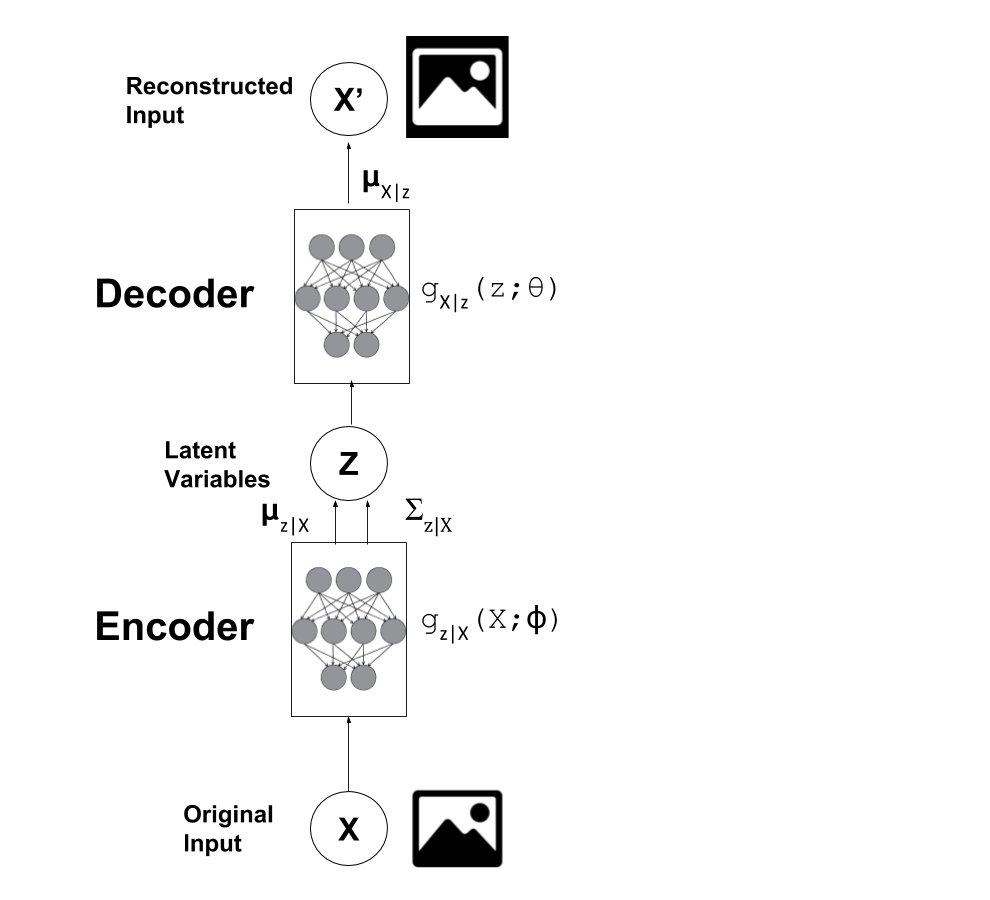
Figure 1: Vanilla Variational Autoencoder

After our VAE has been fully trained, it's easy to see how we can just use the "encoder" to directly help with semi-supervised learning:

1. Train a VAE using all our data points (labelled and unlabelled), and transform our observed data (\(X\)) into the latent space defined by the \(Z\) variables.

2. Solve a standard supervised learning problem on the labelled data using \((Z, Y)\) pairs (where \(Y\) is our label).

Intuitively, the latent space defined by \(z\) should capture some useful information about our data such that it's easily separable in our supervised learning problem. This technique is defined as M1 model in the Kingma paper. As you may have noticed though, step 1 doesn't directly involve any of the \(y\) labels; the steps are disjoint. Kingma also introduces another model "M2" that attempts to solve this problem.

Extending the VAE for Semi-Supervised Learning (M2 Model)

In the M1 model, we basically ignored our labelled data in our VAE. The M2 model (from the Kingma paper) explicitly takes it into account. Let's take a look at the generative model (i.e. the "decoder"):

where:

• \({\bf x}\) is a vector of our observed variables

• \(f({\bf x}; y, {\bf z}, \theta)\) is a suitable likelihood function to model our output such as a Gaussian or Bernoulli. We use a deep net to approximate it based on inputs \(y, {\bf z}\) with network weights defined by \(\theta\).

• \({\bf z}\) is a vector latent variables (same as vanilla VAE)

• \(y\) is a one-hot encoded categorical variable representing our class labels, whose relative probabilities are parameterized by \({\bf \pi}\).

• \(\text{SimDir}\) is Symmetric Dirichlet distribution with hyper-parameter \(\alpha\) (a conjugate prior for categorical/multinomial variables)

How do we do use this for semi-supervised learning you ask? The basic gist of it is: we will define a approximate posterior function \(q_\phi(y|{\bf x})\) using a deep net that is basically a classifier. However the genius is that we can train this classifier for both labelled and unlabelled data by just training this extended VAE. Figure 2 shows a visualization of the network.

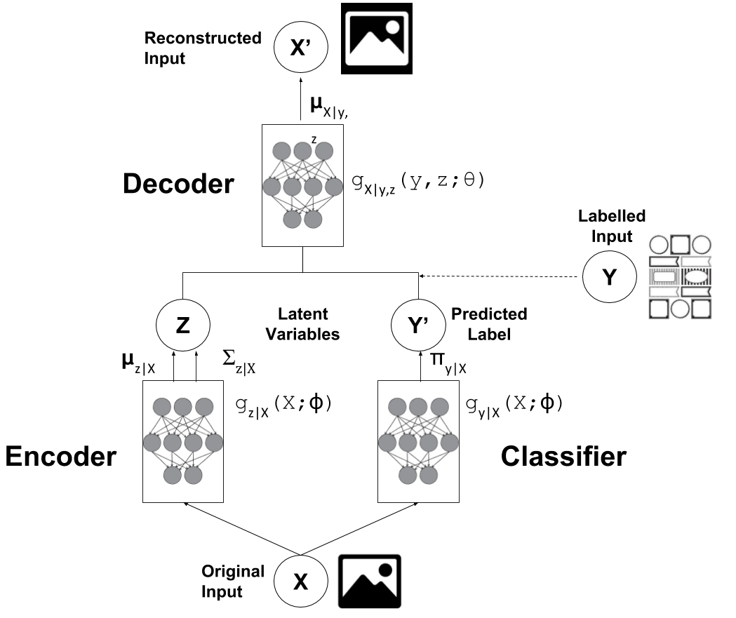
Figure 2: M2 Variational Autoencoder for Semi-Supervised Learning

Now the interesting part is that we have two cases: one where we observe the \(y\) labels and one where we don't. We have to deal with them differently when constructing the approximate posterior \(q\) as well as in the variational objective.

Variational Objective with Unlabelled Data

For any variational inference problem, we need to start with our approximate posterior. In this case, we'll treat \(y, {\bf z}\) as the unknown latent variables, and perform variational inference (i.e. define approximate posteriors) over them. Notice that we excluded \(\pi\) because we don't really care what its posterior is in this case.

We'll assume the approximate posterior \(q_{\phi}(y, {\bf z}|{\bf x})\) has a fully factorized form as such:

where \({\bf \mu}_{\phi}({\bf x}), {\bf \sigma}^2_{\phi}({\bf x}), \pi_{\phi}({\bf X}\)) are all defined by neural networks parameterized by \(\phi\) that we will learn. Here, \(\pi_{\phi}({\bf X})\) should not be confused with our actual parameter \({\bf \pi}\) above, the former is a point-estimate coming out of our network, the latter is a random variable as a symmetric Dirichlet.

From here, we use the ELBO to determine our variational objective for a single data point:

Going through line by line, we factor our \(q_\phi\) function into the separate \(y\) and \({\bf z}\) parts for both the expectation and the \(\log\). Notice we also absorb \(\log p_\theta(y)\) into a constant because \(p(y) = p(y|{\bf \pi})p(\pi)\), a Dirichlet-multinomial distribution, and simplifies to a constant (alternatively, our model's assumption is that \(y\)'s are equally likely to happen).

Next, we notice that some terms form a KL distribution between \(q_{\phi}({\bf z}|{\bf x})\) and \(p_{\theta}({\bf z})\). Then, we group a few terms together and name it \(\mathcal{L}({\bf x}, y)\). This latter term is essentially the same variational objective we used for a vanilla variational autoencoder (sans the reference to \(y\)). Finally, we explicitly write out the expectation with respect to \(y\). I won't write out all the details for how to compute it, for that you can look at my previous post for \(\mathcal{L}({\bf x}, y)\), and the implementation notebooks for the rest. The loss functions are pretty clearly labelled so it shouldn't be too hard to map it back to these equations.

So Equation 6 defines our objective function for our VAE, which will simultaneously train both the \(\theta\) parameters of the "decoder" network as well as the approximate posterior "encoder" \(\phi\) parameters relating to \(y, {\bf z}\).

Variational Objective with Labelled Data

So here's where it gets a bit trickier because this part was glossed over in the paper. In particular, when training with labelled data, you want to make sure you train both the \(y\) and the \({\bf z}\) networks at the same time. It's actually easy to leave out the \(y\) network since you have the observations for \(y\), allowing you to ignore the classifier network.

Now of course the whole point of semi-supervised learning is to learn a mapping using labelled data from \({\bf x}\) to \(y\) so it's pretty silly not to train that part of your VAE using labelled data. So Kingma et al. add an extra loss term initially describing it as a fix to this problem. Then, they add an innocent throw-away line that this actually can be derived by performing variational inference over \(\pi\). Of course, it's actually true (I think) but it's not that straightforward to derive! Well, I worked out the details, so here's my presentation of deriving the variational objective with labelled data.

Updated (2018-10): After receiving some great questions from a few readers, I've taken another look at this and I believe I have a more sensible derivation. See Appendix B below.

For the case when we have both \((x,y)\) points, we'll treat both \(z\) and \({\bf \pi}\) as unknown latent variables and perform variational inference for both \(\bf{z}\) and \({\bf \pi}\) using a fully factorized posterior dependent only on \({\bf x}\).

Remember we can define our approximate posteriors however we want, so we explicitly choose to have \({\bf \pi}\) to depend only on \({\bf x}\) and not on our observed \(y\). Why you ask? It's because we want to make sure our \(\phi\) parameters of our classifier are trained when we have labelled data.

As before, we start with the ELBO to determine our variational objective for a single data point \(({\bf x},y)\):

where \(\alpha\) is a hyper-parameter that controls the relative weight of how strongly you want to train the discriminative classified (\(q_\phi(y|{\bf x})\)). In the paper, they set it to \(\alpha=0.1N\)

Going line by line, we start off with the ELBO, expanding all the priors. The one trick we do is instead of expanding the joint distribution of \(y,{\bf \pi}\) conditioned on \(\pi\) (i.e. \(p_{\theta}(y, {\bf \pi}) = p_{\theta}(y|{\bf \pi})p_{\theta}({\bf \pi})\)), we instead expand using the posterior: \(p_{\theta}({\bf \pi}|y)\). The posterior in this case is again a Dirichlet distribution because it's the conjugate prior of \(y\)'s categorical/multinomial distribution.

Next, we just rearrange and factor \(q_\phi\), both in the \(\log\) term as well as the expectation. We notice that the first part is exactly our \(\mathcal{L}\) loss function from above and the rest is a KL divergence between our \(\pi\) posterior and our approximate posterior. The last simplification of the KL divergence is a bit verbose (and hand-wavy) so I've put it in Appendix A.

Training the M2 Model

Using Equations 6 and 8, we can derive a loss function as such (remember it's the negative of the ELBO above):

With this loss function, we just train the network as you would expect. Simply grab a mini-batch, compute the needed values in the network (i.e. \(q(y|{\bf x}), q(z|{\bf x}), p({\bf x}|y, z)\)), compute the loss function above using the appropriate summation depending on if you have labelled or unlabelled data, and finally just take the gradients to update our network parameters \(\theta, \phi\). The network is remarkably similar to a vanilla VAE with the addition of the posterior on \(y\), and the additional terms to the loss function. The tricky part is dealing with the two types of data (labelled and unlabelled), which I explain in the implementation notes below.

Implementation Notes

The notebooks I used are here on Github. I made one notebook for each experiment, so it should be pretty easy for you to look around. I didn't add as many comments as some of my previous notebooks but I think the code is relatively clean and straightforward so I don't think you'll have much trouble understanding it.

Variational Autoencoder Implementations (M1 and M2)

The architectures I used for the VAEs were as follows:

• For \(q(y|{\bf x})\), I used the CNN example from Keras, which has 3 conv layers, 2 max pool layers, a softmax layer, with dropout and ReLU activation.

• For \(q({\bf z}|{\bf x})\), I used 3 conv layers, and 2 fully connected layers with batch normalization, dropout and ReLU activation.

• For \(p({\bf x}|{\bf z})\) and \(p({\bf x}|y, {\bf z})\), I used a fully connected layer, followed by 4 transposed conv layers (the first 3 with ReLU activation the last with sigmoid for the output).

The rest of the details should be pretty straight forward if you look at the notebook.

The one complication that I had was how to implement the training of the M2 model because you need to treat \(y\) simultaneously as an input and an output depending if you have labelled or unlabelled data. I still wanted to use Keras and didn't want to go as low level as TensorFlow, so I came up with a workaround: train two networks (with shared layers)!

So basically, I have one network for labelled data and one for unlabelled data. They both share all the same components (\(q(y|{\bf x}), q(z|{\bf x}), p({\bf x}|y, z)\)) but differ in their input/output as well as loss functions. The labelled data has input \(({\bf x}, y)\) and output \(({\bf x'}, y')\). \(y'\) corresponds to the predictions from the posterior, while \({\bf x'}\) corresponds to the decoder output. The loss function is Equation 8 with \(\alpha=0.1N\) (not the one I derived in Appendix A). For the unlabelled case, the input is \({\bf x}\) and the output is the predicted \({\bf x'}\).

For the training, I used the train_on_batch() API to train the first network on a random batch of labelled data, followed by the second on unlabelled data. The batches were sized so that the epochs would finish at the same time. This is not strictly the same as the algorithm from the paper but I'm guessing it's close enough (also much easier to implement because it's in Keras). The one cute thing that I did was use vanilla tqdm to mimic the keras_tqdm so I could get a nice progress bar. The latter only works with the regular fit methods so it wasn't very useful.

Comparison Implementations

In the results below I compared a semi-supervised VAE with several other ways of dealing with semi-supervised learning problems:

• PCA + SVM: Here I just ran principal component analysis on the entire image set, and then trained a SVM using a PCA-transformed representation on only the labelled data.

• CNN: A vanilla CNN using the Keras CNN example trained only on labelled data.

• Inception: Here I used a pre-trained Inception network available in Keras. I pretty much just used the example they had which adds a global average pooling layer, a dense layer, followed by a softmax layer. Trained only on the labelled data while freezing all the original pre-trained Inception layers. I didn't do any fine-tuning of the Inception layers.

Semi-supervised Results

The datasets I used were MNIST and CIFAR10 with stratified sampling on the training data to create the semi-supervised dataset. The test sets are the ones included with the data. Here are the results for MNIST:

The M2 model was only run for \(N=1000\) (mostly because I didn't really want to rearrange the code). From the MNIST results table, we really see the the M2 model shine where at a comparable sample size, all the other methods have much lower performance. You need to get to \(N=5000\) before the CNN gets in the same range. Interestingly at \(N=100\) the models that make use of the unlabelled data do better than a CNN which has so little training data it surely is not learning to generalize. Next, onto CIFAR 10 results shown in Table 2.

Again I only train M2 on \(N=1000\). The CIFAR10 results show another story. Clearly the pre-trained Inception network is doing the best. It's pre-trained on Imagenet which is very similar to CIFAR10. You have to get to relatively large sample sizes before even the CNN starts approaching the same accuracy.

The M1/M2 results are quite poor, not even beating out PCA in most cases! My reasoning here is that the CIFAR10 dataset is too complex for the VAE model. That is, when I look at the images generated from it, it's pretty hard for me to figure out what the label should be. Take a look at some of the randomly generated images from my M2 model:

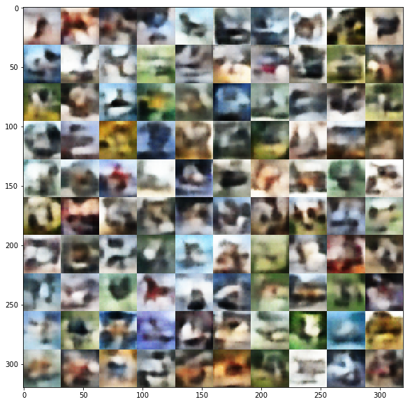
Figure 3: Images generated from M2 VAE model trained on CIFAR data.

Other people have had similar problems. I suspect the \({\bf z}\) Gaussian latent variables are not powerful enough to encode the complexity of the CIFAR10 dataset. I've read somewhere that the unimodal nature of the latent variables is thought to be quite limiting, and here I guess we see that is the case. I'm pretty sure more recent research has tried to tackle this problem so I'm excited to explore this phenomenon more later.

Conclusion

As I've been writing about for the past few posts, I'm a huge fan of scalable probabilistic models using deep learning. I think it's both elegant and intuitive because of the probabilistic formulation. Unfortunately, VAEs using Gaussians as the latent variable do have limitations, and obviously they are not quite the state-of-the-art in generative models (i.e. GANs seem to be the top dog). In any case, there is still a lot more recent research in this area that I'm going to follow up on and hopefully I'll have something to post about soon. Thanks for reading!

Further Reading

• Previous Posts: Variational Autoencoders, A Variational Autoencoder on the SVHN dataset, Variational Bayes and The Mean-Field Approximation, Maximum Entropy Distributions

• Wikipedia: Semi-supervised learning, Variational Bayesian methods, Kullback-Leibler divergence

• "Variational Inference: Foundations and Modern Methods", Blei, Ranganath, Mohamed, NIPS 2016 Tutorial.

• "Semi-supervised Learning with Deep Generative Models", Kingma, Rezende, Mohamed, Welling, https://arxiv.org/abs/1406.5298

• Github report for "Semi-supervised Learning with Deep Generative Models", https://github.com/dpkingma/nips14-ssl/

Appendix A: KL Divergence of \(q_\phi({\bf \pi}|{\bf x})||p_{\theta}({\bf \pi}|y)\)

Notice that the two distributions in question are both Dirichlet distributions:

where \(\alpha_p, \alpha_q\) are scalar constants, and \({\bf c}_y\) is a vector with 0's and a single 1 representing the categorical observation of \(y\). The latter distribution is just the conjugate prior of a single observation of a categorical variable \(y\), whereas the former is basically just something we picked out of convenience (remember it's the posterior approximation that we get to choose).

Let's take a look at the formula for KL divergence between two Dirichlets distributions parameterized by vectors \({\bf \alpha}\) and \({\bf \beta}\):

where \(\alpha_0=\sum_k \alpha_k\) and \(\beta_0=\sum_k \beta_k\), and \(\psi\) is the Digamma function.

Substituting Equation A.1 into A.2, we have:

Here, most of the Gamma functions are just constants so we can absorb them into a constant. Okay, here's where it gets a bit hand wavy (it's the only way I could figure out how to simplify the equation to what it had in the paper). We're going to pick a big \(\alpha_q\) and a small \(\alpha_p\). Both are hyper parameters so we can freely do as we wish. With this assumption, we're going to progressively simplify and approximate Equation A.3:

This is quite a mouthful to explain since I'm just basically waving my hand to get to the final expression. First, we drop the Gamma function in the second term and upper bound it by a new constant \(K_3\) because our \(\alpha_q\) is large, its the gamma function is always positive. Next, we drop \(\alpha_p\) since it's small (let's just make it arbitrarily small). We then drop \(\psi(\alpha_q)\), a constant, because when we expand it out we get a constant (recall \(\sum_{k=1}^K \pi_{\phi, k}({\bf x}) = 1\)).

Now we're getting somewhere! Since \(\alpha_q\) is again large the Digamma function is upper bounded by \(\log(x)\) when \(x>0.5\), so we'll just make this substitution. Finally, we get something that looks about right. We just rearrange a bit and two non-constant terms involving entropy of \(q\) and the probability of a categorical variable with parameter \(\pi({\bf x})\). We just upper bound the expression by dropping the \(-H(q)\) term since entropy is always positive to get us to our final term \(-\log(q(y|{\bf x}))\) that Kingma put in his paper. Although, one thing I couldn't quite get to is the additional constant \(\alpha\) that is in front of \(\log(q(y|{\bf x}))\).

Admittedly, it's not quite precise, but it's the only way I figured out how to derive his expression without just arbitrarily adding an extra term to the loss function (why work out any math when you're going to arbitrarily add things to the loss function?). Please let me know if you have a better way of deriving this equation.

Appendix B: Updated Derivation of Variational Objective with Labelled Data

First, we'll re-write the factorization of our generative model from Equation 4 to explicitly show \({\bf \pi}\):

Notice a couple of things:

1. In our generative model, our output (\({\bf x}\)) only depends directly on \(y, {\bf z}\), not \(\pi\).

2. We are now emphasizing the relationship between \(y\) and \(\pi\), where \(y\) depends on \(\pi\).

Next, we'll have to change our posterior approximation a bit:

Notice that we're using \(q(\pi|{\bf x})\) instead of \(q(y|{\bf x})\). This requires some explanation. Recall, our approximation network (\(q(y|{\bf x})\)) is outputting the parameters for our categorical variable \(y\), call it \(\pi_{q(y|{\bf x})}\), this clearly does not define a distribution over \(\pi\); it's actually just a point estimate of \(\pi\). So how do we get \(q(\pi|{\bf x})\)? We take this point estimate and assume it defines a Dirac delta distribution! In other words, it's density is zero everywhere except at a single point and its integral over the entire support is \(1\). This of course is some sort of hack to make the math work out but I think it's a bit more elegant than throwing an extra loss term or the hand-waving I did above.

So now that we have re-defined our posterior approximation, we go through our ELBO equation as before:

We expand our generative model and posterior approximation according to the factorizations in Equations B.1 and B.2, and then group them together into their respective expectations. Finally, we see that the \(-\mathcal{L}({\bf x},y)\) terms appear as before along with a KL divergence term. Up until here, the derivation should resemble everything we've done before.

From here, we have to deal with the KL divergence term... by getting rid of it! How can we do this? Well, we really can't. The KL divergence term is actually \(-\infty\) (by method of taking the limit implicit in the Dirac delta distribution) because the divergence between a symmetric Dirichlet distribution (\(p(\pi)\)) and a point estimate using a Dirac delta distribution (\(q(\pi|{\bf x})\)) is infinite. However, looking at it from another angle because we chose a Dirac delta distribution for the posterior approximation, the divergence will always be infinite. So if it's always infinite, why even care about it in our loss function? Hopefully, you kind of buy this argument:

Continuing on (after getting rid of the KL divergence term), we utilize our selection of \(q(\pi|{\bf x})\) as a Dirac delta distribution:

We can see the Dirac delta simplifies the expectation significantly, which just "filters" out the logarithm from the integral. Next, we expand out \(p(y|\pi_{q(y|{\bf x})})\) with the PDF of a categorical variable at a given value of \(y\) (\(I\) is the indicator function). The indicator function essentially filters out the proportion for the observed \(y\) value, which is just the PDF of \(q(y|{\bf x})\), our approximate posterior as required.