Variational Bayes and The Mean-Field Approximation

Brian Keng

2017-04-03 08:02

This post is going to cover Variational Bayesian methods and, in particular, the most common one, the mean-field approximation. This is a topic that I've been trying to understand for a while now but didn't quite have all the background that I needed. After picking up the main ideas from variational calculus and getting more fluent in manipulating probability statements like in my EM post, this variational Bayes stuff seems a lot easier.

Variational Bayesian methods are a set of techniques to approximate posterior distributions in Bayesian Inference. If this sounds a bit terse, keep reading! I hope to provide some intuition so that the big ideas are easy to understand (which they are), but of course we can't do that well unless we have a healthy dose of mathematics. For some of the background concepts, I'll try to refer you to good sources (including my own), which I find is the main blocker to understanding this subject (admittedly, the math can sometimes be a bit cryptic too). Enjoy!

Variational Bayesian Inference: An Overview

Before we get into the nitty-gritty of it all, let's just go over at a high level what we're trying to do. First, we're trying to perform Bayesian inference, which basically means given a model, we're trying to find distributions for the unobserved variables (either parameters or latent variables since they're treated the same). This problem usually involves hard-to-solve integrals with no analytical solution.

There are two main avenues to solve this problem. The first is to just get a point-estimate for each of the unobserved variables (either MAP or MLE) but this is not ideal since we can't quantify the uncertainty of the unknown variables (and is against the spirit of Bayesian analysis). The other aims to find a (joint) distribution of each unknown variable. With a proper distribution for each variable, we can do a whole bunch of nice Bayesian analysis like the mean, variance, 95% credible interval etc.

One good but relatively slow method for finding a distribution is to use MCMC (a simulation technique) to iteratively draw samples that eventually give you the shape of the joint distribution of the unknown variables. Another method is to use variational Bayes, which helps to find an approximation of the distribution in question. With variational Bayes, you only get approximation but it's in analytical form (read: easy to compute). So long as your approximation is pretty good, you can do all the nice Bayesian analysis you like, and the best part is it's relatively easy to compute!

The next example shows a couple of Bayesian inference problems to make things more concrete.

Example 1: Bayesian Inference Problems

Fitting a univariate Gaussian with unknown mean and variance: Given observed data \(X=\{x_1,\ldots, x_N\}\), we wish to model this data as a normal distribution with parameters \(\mu,\sigma^2\) with a normally distributed prior on the mean and an inverse-gamma distributed prior on the variance. More precisely, our model can be defined as:

\begin{align*} \mu &\sim \mathcal{N}(\mu_0, (\kappa_0\tau)^{-1}) \\ \tau &\sim \text{Gamma}(a_0, b_0) \\ x_i &\sim \mathcal{N}(\mu, \tau^{-1}) \\ \tag{1} \end{align*}

where the hyperparameters \(\mu_0, \kappa_0, a_0, b_0\) are given and \(\tau\) is the inverse of the variance known as the precision. In this model, the parameter variables \(\mu,\tau\) are unobserved, so we would use variational Bayes to approximate the posterior distribution \(q(\mu, \tau) \approx p(\mu, \tau | x_1, \ldots, x_N)\).
Bayesian Gaussian Mixture Model: A Bayesian Gaussian mixture model with \(K\) mixture components and \(N\) observations \(\{x_1,\ldots,x_N\}\), latent categorical variables \(\{z_1,\ldots,z_N\}\), parameters \({\mu_i, \Lambda_i, \pi}\) and hyperparameters \({\mu_0, \beta_0, \nu_0, W_0, \alpha_0}\), can be described as such:

\begin{align*} \pi &\sim \text{Symmetric-Dirichlet}_K(\alpha_0) \\ \Lambda_{k=1,\ldots,K} &\sim \mathcal{W}(W_0, \nu_0) \\ \mu_{k=1,\ldots,K} &\sim \mathcal{N}(\mu_0, (\beta_0\Lambda_k)^{-1}) \\ z_i &\sim \text{Categorical}(\pi) \\ x_i &\sim \mathcal{N}(\mu_{z_i}, \Lambda_{z_i}^{-1}) \\ \tag{2} \end{align*}

Notes:
- \(\mathcal{W}\) is the Wishart distribution, which is the generalization to multiple dimensions of the gamma distribution. It's used for the prior on the covariance matrix for our multivariate normal distribution. It's also a conjugate prior of the precision matrix (the inverse of the covariance matrix).
- \(\text{Symmetric-Dirichlet}\) is a Dirichlet distribution which is the conjugate prior of a categorical variable (or equivalently a multinomial distribution with a single observation).
In this case, you would want to (ideally) find an approximation to the joint distribution posterior (including both parameters and latent variables): \(q(\mu_1,\ldots,\mu_K, \Lambda_1,\ldots, \Lambda_K, \pi, z_1, \ldots, z_N)\) that approximates the true posterior in all of these latent variables and parameters.

Now that we know our problem, next thing we need to is define what it means to be a good approximation. In many of these cases, the Kullback-Leibler divergence (KL divergence) is a good choice, which is non-symmetric measure of the difference between two probability distributions \(P\) and \(Q\). We'll discuss this in detail in the box below, but the setup will be \(P\) as the true posterior distribution, and \(Q\) being the approximate distribution, and with a bit of math, we want to find an iterative algorithm to compute \(Q\).

In the mean-field approximation (a common type of variational Bayes), we assume that the unknown variables can be partitioned so that each partition is independent of the others. Using KL divergence, we can derive mutually dependent equations (one for each partition) that define the shape of \(Q\). The resultant \(Q\) function then usually takes on the form of well-known distributions that we can easily analyze. The leads to an easy-to-compute iterative algorithm (similar to the EM algorithm) where we use all other previously calculated partitions to derive the current one in an iterative fashion.

To summarize, variational Bayes has these ideas:

The Bayesian inference problem of finding a posterior on the unknown variables (parameters and latent variables) is hard and usually can't be solved analytically.
Variational Bayes solves this problem by finding a distribution \(Q\) that approximates the true posterior \(P\).
It uses KL-divergence as a measure of how well our approximation fits the true posterior.
The mean-field approximation partitions the unknown variables and assumes each partition is independent (a simplifying assumption).
With some (long) derivations, we can find an algorithm that iteratively computes the \(Q\) distributions for a given partition by using the previous values of all the other partitions.

Now that we have an overview of this process, let's see how it actually works.

Kullback-Leibler Divergence

Kullback-Leibler divergence (aka information gain) is a non-symmetric measure of the difference between two probability distributions \(P\) and \(Q\). It is defined for discrete and continuous probability distributions as such:

\begin{align*} D_{KL}(P||Q) &= \sum_i P(i) \log \frac{P(i)}{Q(i)} \\ D_{KL}(P||Q) &= \int_{-\infty}^{\infty} p(x) \log \frac{p(x)}{q(x)} dx \\ \tag{3} \end{align*}

where \(p\) and \(q\) denote the densities of \(P\) and \(Q\).

There are several ways to intuitively understand KL-divergence, but let's use information entropy because I think it's a bit more intuitive.

KL Divergence as Information Gain

To quickly summarize, entropy is the average amount of information or "surprise" for a probability distribution 1. Entropy is defined as for both discrete and continuous distributions:

\begin{align*} H(P) &:= E_P[I_P(X)] = -\sum_{i=1}^n P(i) \log(P(i)) \\ H(P) &:= E_P[I_P(X)] = - \int_{-\infty}^{\infty} p(x)\log(p(x)) dx \\ \tag{4} \end{align*}

An intuitive way to think about entropy is the (theoretical) minimum number of bits you need to encode an event (or symbol) drawn from your probability distribution (see Shannon's source coding theorem). For example, for a fair eight-sided die, each outcome is equi-probable, so we would need \(\sum_1^8 -\frac{1}{8}log_2(\frac{1}{8}) = 3\) bits to encode the roll on average. On the other hand, if we have a weighted eight-sided die where "8" came up 40 times more often than the other numbers, we would theoretically need about 1 bit to encode the roll on average (to get close, we would assign "8" to a single bit 0, and others to something like 10, 110, 111 ... using a prefix code).

In this way of viewing entropy, we're using the assumption that our symbols are drawn from probability distribution \(P\) to get as close as we can to the theoretical minimum code length. Of course, we rarely have an ideal encoding. What would our average message length (i.e. entropy) be if we used the ideal symbols from another distribution such as \(Q\)? In that case, it would just be \(H(P,Q) := E_P[I_Q(X)] = E_P[-\log(Q(X))]\), which is also called the cross entropy of \(P\) and \(Q\). Of course, it would be larger than the ideal encoding, thus we would increase the average message length. In other words, we need more information (or bits) to transmit a message from the \(P\) distribution using \(Q\)'s code.

Thus, KL divergence can be viewed as this average extra-message length we need when we wrongly assume the probability distribution, using \(Q\) instead of \(P\):

\begin{align*} D_{KL}(P||Q) &= H(P,Q) - H(P)\\ &= -\sum_{i=1}^n P(i) \log(Q(i)) + \sum_{i=1}^n P(i) \log(P(i)) \\ &= \sum_{i=1}^n P(i) \log\frac{P(i)}{Q(i)} \\ \tag{5} \end{align*}

You can probably already see how this is a useful objective to try to minimize. If we have some theoretic minimal distribution \(P\), we want to try to find an approximation \(Q\) that tries to get as close as possible by minimizing the KL divergence.

Forward and Reverse KL Divergence

One thing to note about KL divergence is that it's not symmetric, that is, \(D_{KL}(P||Q) \neq D_{KL}(Q||P)\). The former is called forward KL divergence, while the latter is called reverse KL divergence. Let's start by looking at forward KL. Taking a closer look at equation 5, we can see that when \(P\) is large and \(Q \rightarrow 0\), the logarithm blows up. This implies when choosing our approximate distribution \(Q\) to minimize forward KL divergence, we want to "cover" all the non-zero parts of \(P\) as best we can. Figure 1 shows a good visualization of this.

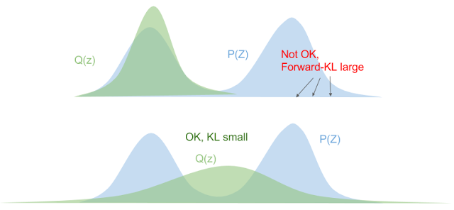
Forward KL Divergence (source: `Eric Jang's Blog <http://blog.evjang.com/2016/08/variational-bayes.html>`__)

Figure 1: Forward KL Divergence (source: Eric Jang's Blog)

From Figure 1, our original distribution \(P\) is multimodal, while our approximate one \(Q\) is bell shaped. In the top diagram, if we just try to "cover" one of the humps, then the other hump of \(P\) has a large mass with a near-zero value of \(Q\), resulting in a large KL divergence. In the bottom diagram, we can see that if we try to "cover" both humps by placing \(Q\) somewhere in between, we'll get a smaller forward KL. Of course, this has other problems like the maximum density (center of \(Q\)) is now at a point that has low density in the original distribution.

Now, let's take a look at reverse KL, where \(P\) is still our theoretic distribution we're trying to match and \(Q\) is our approximation:

\begin{align*} D_{KL}(Q||P) = \sum_{i=1}^n Q(i) \log\frac{Q(i)}{P(i)} \\ \tag{6} \end{align*}

From Equation 6, we can see that the opposite situation occurs. If \(P\) is small, we want \(Q\) to be (proportionally) small too or the ratio might blow up. Additionally, when \(P\) is large, it doesn't cause us any particular problems because it just means the ratio is close to 0. Figure 2 shows this visually.

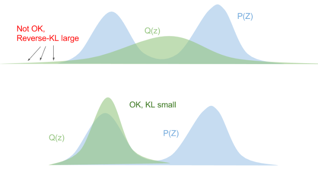
Reverse KL Divergence (source: `Eric Jang's Blog <http://blog.evjang.com/2016/08/variational-bayes.html>`__)

Figure 2: Reverse KL Divergence (source: Eric Jang's Blog)

From Figure 2, we see in the top diagram that if we try to fit our unimodal distribution "in-between" the two maxima of \(P\), the tails cause us some problems where \(P\) drops off much faster than \(Q\) causing the ratio at those points to blow up. The bottom diagram shows a better fit according to reverse KL, the tails of \(P\) and \(Q\) drop off at a similar rate, not causing any issues. Additionally, since \(Q\) matches one of the mode of our \(P\) distribution well, the logarithm factor will be close to zero, also making for a better reverse KL fit. Reverse KL also has the nice tendency to make our \(Q\) distribution matches at least one of the modes of \(P\), which is really the best we could hope for with the shape of our approximation.

In our use of KL divergence, we'll be using reverse KL divergence, not only because of the nice properties above, but for the more practical reason that the math works out nicely :p

From KL divergence to Optimization

Remember what we're trying to accomplish: we have some intractable Bayesian inference problem \(P(\theta|X)\) we're trying to compute, where \(\theta\) are the unobserved variables (parameters or latent variables) and \(X\) are our observed data. We could try to compute it directly using Bayes theorem (continuous version, where \(p\) is the density of distribution \(P\)):

\begin{align*} p(\theta|X) &= \frac{p(X, \theta)}{p(X)} \\ &= \frac{p(X|\theta)p(\theta)}{\int_{-\infty}^{\infty} p(X|\theta)p(\theta) d\theta} \\ &= \frac{\text{likelihood}\cdot\text{prior}}{\text{marginal likelihood}} \\ \tag{7} \end{align*}

However, this is generally difficult to compute because of the marginal likelihood (sometimes called the evidence). But what if we didn't have to directly compute the marginal likelihood and instead only needed the likelihood (and prior)?

This idea leads us to the two commonly used methods to solve Bayesian inference problems: MCMC and variational inference. You can check out my previous post on MCMC but in general it's quite slow since it involves repeated sampling but your approximation can get arbitrarily close to the actual distribution (given enough time). Variational inference on the other hand is a strict approximation that is much faster because it is an optimizing problem. It also can quantify the lower bound on the marginal likelihood, which can help with model selection.

Now going back to our problem, we want to find an approximate distribution \(Q\) that minimizes the (reverse) KL divergence. Starting from reverse KL divergence, let's do some manipulation to get to an equation that's easy to interpret (using continuous version here), where our approximate density is \(q(\theta)\) and our theoretic one is \(p(\theta|X)\):

\begin{align*} D_{KL}(Q||P) &= \int_{-\infty}^{\infty} q(\theta) \log\frac{q(\theta)}{p(\theta|X)} d\theta \\ &= \int_{-\infty}^{\infty} q(\theta) \log\frac{q(\theta)}{p(\theta,X)} d\theta + \int_{-\infty}^{\infty} q(\theta) \log{p(X)} d\theta \\ &= \int_{-\infty}^{\infty} q(\theta) \log\frac{q(\theta)}{p(\theta,X)} d\theta + \log{p(X)} \\ \tag{8} \end{align*}

Where we're using Bayes theorem on the second line and the RHS integral simplifies because it's simply integrating over the support of \(q(\theta)\) (\(\log p(X)\) is not a function of \(\theta\) so it factors out). Rearranging we get:

\begin{align*} \log{p(X)} &= D_{KL}(Q||P) - \int_{-\infty}^{\infty} q(\theta) \log\frac{q(\theta)}{p(\theta,X)} d\theta \\ &= D_{KL}(Q||P) + \mathcal{L}(Q) \tag{9} \end{align*}

where \(\mathcal{L}\) is called the (negative) variational free energy 2, NOT the likelihood (I don't like the choice of symbols either but that's how it's shown in most texts). Recall that the evidence on the LHS is constant (for a given model), thus if we maximize the variational free energy \(\mathcal{L}\), we minimize (reverse) KL divergence as required.

This is the crux of variational inference: we don't need to explicitly compute the posterior (or the marginal likelihood), we can solve an optimization problem by finding the right distribution \(Q\) that best fits our variational free energy. Notice that we don't need to compute the marginal likelihood either, this is a big win because the likelihood and prior are usually easily specified with the marginal likelihood intractable. Note that we need to find a function, not just a point, that maximizes \(\mathcal{L}\), which means we need to use variational calculus (see my previous post on the subject), hence the name "variational Bayes".

The Mean-Field Approximation

Before we try to derive the functional form of our \(Q\) functions, let's just explicitly state some of our notation because it's going to get a bit confusing. In the previous section, I used \(\theta\) to represent the unknown variables. In general, we can have \(N\) unknown variables so \(\theta = (\theta_1, \ldots, \theta_N)\) and Equation 8 and 9 will have multiple integrals (or summations for discrete variables), one for each \(\theta_i\). I'll use \(\theta\) to represent \(\theta_1, \ldots, \theta_N\) where it is clear just to reduce the verbosity and explicitly write it out when we want to do something special with it.

Okay, so now that's cleared up, let's move on to the mean-field approximation. The approximation is a simplifying assumption for our \(Q\) distribution, which partitions the variables into independent parts (I'm just going to show one variable per partition but you can have as many per partition as you want):

\begin{equation*} p(\theta|X) \approx q(\theta) = q(\theta_1, \ldots, \theta_n) = \prod_{i=1}^N q_i(\theta_i) \tag{10} \end{equation*}

Deriving the Functional Form of \(q_j(\theta_j)\)

From Equation 10, we can plug it back into our variational free energy \(\mathcal{L}\) and try to derive the functional form of \(q_j\) using variational calculus 3. Let's start with \(\mathcal{L}\) and try to re-write it isolating the terms for \(q_j(\theta_j)\) in hopes of taking a functional derivative afterwards to find the optimal form of the function. Note that \(\mathcal{L}\) is a functional that depends on our approximate densities \(q_1, \ldots, q_N\).

\begin{align*} \mathcal{L[q_1, \ldots, q_N]} &= - \int_{\theta_1, \ldots, \theta_N} [\prod_{i=1}^N q_i(\theta_i)] \log\frac{[\prod_{k=1}^N q_k(\theta_k)]}{p(\theta,X)} d\theta_1 \ldots d\theta_n \\ &= \int_{\theta_1, \ldots, \theta_N} [\prod_{i=1}^N q_i(\theta_i)] \big[ \log p(\theta,X) - \sum_{k=1}^N \log q_k(\theta_k) \big] d\theta_1 \ldots d\theta_n \\ &= \int_{\theta_j} q_j(\theta_j) \int_{\theta_{m | m \neq j}} [\prod_{i\neq j} q_i(\theta_i)] \big[ \log p(\theta,X) - \sum_{k=1}^N \log q_k(\theta_k) \big] d\theta_1 \ldots d\theta_n \\ &= \int_{\theta_j} q_j(\theta_j) \int_{\theta_{m | m \neq j}} [\prod_{i\neq j} q_i(\theta_i)] \log p(\theta,X) d\theta_1 \ldots d\theta_n \\ &\phantom{=}- \int_{\theta_j} q_j(\theta_j) \int_{\theta_{m | m \neq j}} [\prod_{i\neq j} q_i(\theta_i)] \sum_{k=1}^N \log q_k(\theta_k) d\theta_1 \ldots d\theta_n \\ \tag{11} \end{align*}

where I'm using a bit of convenience notation in the integral index (\(\theta_m|m\neq j\)) so I don't have to write out the "\(...\)". So far, we've just factored out \(q_j(\theta_j)\) and multiplied out the inner term \(\log p(\theta, X) - \sum_{i=k}^N \log q_k(\theta_k)\). In anticipation of the next part, we'll define some notation for an expectation across all variables except \(j\) as:

\begin{align*} E_{m|m\neq j}[\log p(\theta,X)] = \int_{\theta_{m | m \neq j}} [\prod_{i\neq j} q_i(\theta_i)] \log p(\theta,X) d\theta_1 \ldots, d\theta_{j-1}, d\theta_{j+1}, \ldots, d\theta_n \\ \tag{12} \end{align*}

which you can see is just an expectation across all variables except for \(j\). Continuing on from Equation 11 using this expectation notation and expanding the second term out:

\begin{align*} \mathcal{L}[q_1, \ldots, q_N] &= \int_{\theta_j} q_j(\theta_j) E_{m|m\neq j}[\log p(\theta, X)] d\theta_j \\ &\phantom{=}- \int_{\theta_j} q_j(\theta_j) \log q_j(\theta_j) \int_{\theta_{m | m \neq j}} [\prod_{i\neq j} q_i(\theta_i)] d\theta_1 \ldots d\theta_n \\ &\phantom{=}- \int_{\theta_j} q_j(\theta_j) d\theta_j \int_{\theta_{m | m \neq j}} [\prod_{i\neq j} q_i(\theta_i)] \sum_{k\neq j} \log q_k(\theta_k) d\theta_1 \ldots, d\theta_{j-1}, d\theta_{j+1}, \ldots, d\theta_n \\ &= \int_{\theta_j} q_j(\theta_j) E_{m|m\neq j}[\log p(\theta, X)] d\theta_j - \int_{\theta_j} q_j(\theta_j) \log q_j(\theta_j) d\theta_j\\ &\phantom{=}- \int_{\theta_{m | m \neq j}} [\prod_{i\neq j} q_i(\theta_i)] \sum_{k\neq j} \log q_k(\theta_k) d\theta_1 \ldots, d\theta_{j-1}, d\theta_{j+1}, \ldots, d\theta_n \\ &= \int_{\theta_j} q_j(\theta_j) \big[E_{m|m\neq j}[\log p(\theta, X)] - \log q_j(\theta_j)\big] d\theta_j \\ &\phantom{=}- G[q_1, \ldots, q_{j-1}, q_{j+1}, \ldots, q_{N}] \\ \tag{13} \end{align*}

where we're integrating probability density functions over their entire support in a couple of places, which simplifies a few of the expressions to \(1\). It's a bit confusing because of all the indices but just take your time to follow which index we're pulling out of which summation/integral/product and you shouldn't have too much trouble (unless I made a mistake!). At the end, we have a functional that consists of a term made up only of \(q_j(\theta_j)\) and \(E_{m|m\neq j}[\log p(\theta, X)]\), and another term with all the other \(q_i\) functions.

Putting together the Lagrangian for Equation 13, we get:

\begin{align*} \mathcal{L}[q_1, \ldots, q_N] - \sum_{i=1}^N \lambda_i \int_{\theta_i} q_i(\theta_i) d\theta_i \\ \tag{14} \end{align*}

where the terms in the summation are our usual probabilistic constraints that the \(q_i(\theta_i)\) functions must be probability density functions.

Taking the functional derivative of Equation 14 with respect to \(q_j(\theta_j)\) using the Euler-Lagrange Equation, we get:

\begin{align*} \frac{\delta \mathcal{L}[q_1, \ldots, q_N]}{\delta q_j(\theta)} &= \frac{\partial}{\partial q_j}\big[ q_j(\theta_j) \big[E_{m|m\neq j}[\log p(\theta, X)] - \log q_j(\theta_j)\big] - \lambda_j q_j(\theta_j) \big] \\ &= E_{m|m\neq j}[\log p(\theta, X)] - \log q_j(\theta_j) - 1 - \lambda_j \\ \tag{15} \end{align*}

In this case, the functional derivative is just the partial derivative with respect to \(q_j(\theta_j)\) of what's "inside" the integral. Setting to 0 and solving for the form of \(q_j(\theta_j)\):

\begin{align*} \log q_j(\theta_j) &= E_{m|m\neq j}[\log p(\theta, X)] - 1 - \lambda_j \\ &= E_{m|m\neq j}[\log p(\theta, X)] + \text{const} \\ q_j(\theta_j) &= \frac{e^{E_{m|m\neq j}[\log p(\theta, X)]}}{Z_j} \\ \tag{16} \end{align*}

where \(Z_j\) is a normalization constant. The constant isn't too important because we know that \(q_j(\theta_j)\) is a density so usually we can figure it out after the fact.

Equation 16 finally gives us the functional form (actually a template of the functional form). What usually ends up happening is that after plugging in \(E_{m|m\neq j}[\log p(\theta, X)]\), the form of Equation 16 matches a familiar distribution (e.g. Normal, Gamma etc.), and the normalization constant \(Z\) can be derived by inspection. We'll see this play out in the next section.

Taking a step back, let's see how this helps us accomplish our goal. Recall, we wanted to maximize our variational free energy \(\mathcal{L}\) (Equation 9), which in turn finds a \(q(\theta)\) that minimizes KL divergence to the true posterior \(p(\theta|X)\). Using the mean-field approximation, we broke up \(q(\theta)\) (Equation 10) into partitions \(q_j(\theta_j)\), each of which is defined by Equation 16.

However, the \(q_j(\theta_j)\)'s are interdependent when minimizing them. That is, to compute the optimal \(q_j(\theta_j)\), we need to know the values of all the other \(q_i(\theta_i)\) functions (because of the expectation \(E_{m|m\neq j}[\log p(\theta, X)]\)). This suggests an iterative optimization algorithm:

Start with some random values for each of the parameters of the \(q_j(\theta_j)\) functions.
For each \(q_j\), use Equation 16 to minimize the overall KL divergence by updating \(q_j(\theta_j)\) (holding all the others constant).
Repeat until convergence.

Notice that in each iteration, we are lowering the KL divergence between our \(Q\) and \(P\) distributions, so we're guaranteed to be improving each time. Of course in general we won't converge to a global maximum but it's a heck of a lot easier to compute than MCMC.

Mean-Field Approximation for the Univariate Gaussian

Now that we have a theoretical understanding of how this all works, let's see it in action. Perhaps the simplest case (and I'm using the word "simple" in relative terms here) is the univariate Gaussian with a Gaussian prior on its mean and a inverse Gamma prior on its variance (from Example 1). Let's describe the setup:

\begin{align*} \mu &\sim N(\mu_0, (\kappa_0 \tau)^{-1}) \\ \tau &\sim \text{Gamma}(a_0, b_0) \\ X={x_1, \ldots, x_N} &\sim N(\mu, \tau^{-1}) \\ \tag{17} \end{align*}

where \(\tau\) is the precision (inverse of variance), and we have \(N\) observations (\({x_1, \ldots, x_N}\)). For this particular problem, there is a closed form for the posterior: a Normal-gamma distribution. This means that it doesn't really make sense to compute a mean-field approximation for any reason except pedagogy but that's why we're here right?

Continuing on, we really only need the logarithm of the joint probability of all the variables, which is:

\begin{align*} \log p(X, \mu, \tau) &= \log p(X|\mu, \tau) + \log p(\mu|\tau) + \log p(\tau) \\ &= \frac{N}{2} \log \tau - \frac{\tau}{2} \sum_{i=1}^N (x_i - \mu)^2 \\ &\phantom{=} + \frac{1}{2}\log(\kappa_0 \tau) - \frac{\kappa_0 \tau}{2}(\mu - \mu_0)^2 \\ &\phantom{=} + (a_0 -1) \log \tau - b_0 \tau + \text{const} \tag{18} \end{align*}

I broke out each of the three parts into three lines, so you should be able to easily see how we derived each of the expressions (Normal, Normal, Gamma, respectively). We also just absorbed all the constants into the \(\text{const}\) term.

The Approximation

Now onto our mean-field approximation:

\begin{align*} p(\mu, \tau | X) \approx q(\mu, \tau) := q_{\mu}(\mu)q_{\tau}(\tau) \\ \tag{19} \end{align*}

Continuing on, we can use Equation 16 to find the form of our \(q\) densities. Starting with \(q_{\mu}(\mu)\):

\begin{align*} \log q_{\mu}(\mu) &= E_{\tau}[\log p(X, \mu, \tau)] + \text{const}_1 \\ &= E_{\tau}[\log p(X|\mu, \tau) + \log p(\mu|\tau) + \log p(\tau)] + \text{const}_1 \\ &= E_{\tau}[\log p(X|\mu, \tau) + \log p(\mu|\tau)] + \text{const}_2 \\ &= E_{\tau}\big[\frac{N}{2} \log \tau - \frac{\tau}{2} \sum_{i=1}^N (x_i - \mu)^2 + \frac{1}{2}\log(\kappa_0 \tau) - \frac{\kappa_0 \tau}{2}(\mu - \mu_0)^2 \big] + \text{const}_3 \\ &= -\frac{E_{\tau}[\tau]}{2} \big[ \kappa(\mu - \mu_0)^2 + \sum_{i=1}^N (x_i - \mu)^2 \big] + \text{const}_4 \tag{20} \end{align*}

where we absorb all terms not involving \(\mu\) into the "const" terms (even terms involving only \(\tau\) because it doesn't change with respect to \(\mu\)). You'll notice that Equation 20 is a quadratic function in \(\mu\), implying that it's normally distributed, i.e. \(q_{\mu}(\mu) \sim N(\mu|\mu_N, \tau_N^{-1})\). By completing the square (or using the formula for the sum of two normal distributions), we will find an expression like:

\begin{align*} \log q_{\mu}(\mu) &= -\frac{(\kappa_0 + N)E_{\tau}[\tau]}{2} \big( \mu - \frac{\kappa_0\mu_0 + \sum_{i=1}^N x_i}{\kappa_0 + N} \big)^2 + \text{const}_5 \\ \mu_N &= \frac{\kappa_0\mu_0 + \sum_{i=1}^N x_i}{\kappa_0 + N} \\ \tau_N &= (\kappa_0 + N)E_{\tau}[\tau] \\ \tag{21} \end{align*}

Once we completed the square in Equation 21, we can infer the mean and precision without having to compute all those constants (thank goodness!). Next, we can do the same with \(\tau\):

\begin{align*} \log q_{\tau}(\tau) &= E_{\mu}[\log p(X|\tau, \mu) + \log p(\mu|\tau) + \log p(\tau)] + \text{const}_6 \\ &= E_{\mu}\big[\frac{N}{2} \log \tau - \frac{\tau}{2} \sum_{i=1}^N (x_i - \mu)^2 \\ &\phantom{=} + \frac{1}{2}\log(\kappa_0 \tau) - \frac{\kappa_0 \tau}{2}(\mu - \mu_0)^2 \\ &\phantom{=} + (a_0 -1) \log \tau - b_0 \tau\big] + \text{const}_7 \\ &= (a_0 - 1)\log \tau - b_0\tau + \frac{1}{2}\log \tau + \frac{N}{2} \log \tau \\ &\phantom{=} -\frac{\tau}{2}E_{\mu}\big[\kappa_0(\mu - \mu_0)^2 + \sum_{i=1}^N (x_i - \mu)^2\big] + \text{const}_8 \\ \tag{22} \end{align*}

We can recognize this as a \(\text{Gamma}(\tau|a_N, b_N)\) because the log density is only a function of \(\log\tau\) and \(\tau\). By inspection (and some grouping), we can find the parameters of this Gamma distribution (\(a_N, b_N\)):

\begin{align*} \log q_{\tau}(\tau) &= \big(a_0 + \frac{N + 1}{2} - 1\big)\log\tau \\ &\phantom{=} - \big(b_0 + \frac{1}{2}E_{\mu}\big[\kappa_0(\mu - \mu_0)^2 + \sum_{i=1}^N (x_i - \mu)^2\big] \big)\tau + \text{const}_9 \\ a_N &= a_0 + \frac{N + 1}{2} \\ b_N &= b_0 + \frac{1}{2}E_{\mu}\big[\kappa_0(\mu - \mu_0)^2 + \sum_{i=1}^N (x_i - \mu)^2\big] \\ \tag{23} \end{align*}

Again, we don't have to explicitly compute all the constants which is really nice. Since we know the form of each distribution, the expectation for each of the distributions, \(q(\mu) = N(\mu|\mu_N, \tau_N^{-1})\) and \(q(\tau) = \text{Gamma}(\tau|a_N, b_N)\), is simple:

\begin{align*} E_{q_{\mu}(\mu)}[\mu] &= \mu_N \\ E_{q_{\mu}(\mu)}[\mu^2] &= \frac{1}{\tau_N} + \mu_N^2 \\ E_{q_{\tau}(\tau)}[\tau] &= \frac{a_N}{b_N} \\ \tag{24} \end{align*}

Expanding out Equations 21 and 23 to get our actual update equations:

\begin{align*} \mu_N &= \frac{\kappa_0\mu_0 + \sum_{i=1}^N x_i}{\kappa_0 + N} \\ \tau_N &= (\kappa_0 + N)\frac{a_N}{b_N} \\ a_N &= a_0 + \frac{N + 1}{2} \\ b_N &= b_0 + \frac{\kappa_0}{2}\big( E_{q_{\mu}(\mu)}[\mu^2] + \mu_0^2 - 2E_{q_{\mu}(\mu)}[\mu]\mu_0 \big) \\ &\phantom{=} + \frac{1}{2} \sum_{i=1}^N \big( x_i^2 + E_{q_{\mu}(\mu)}[\mu^2] - 2E_{q_{\mu}(\mu)}[\mu]x_i \big) \\ \tag{25} \end{align*}

where in the \(b_N\) equations, I didn't substitute some of the values from Equation 24 to keep it a bit neater. From this, we can develop a simple algorithm to compute \(q(\mu)\) and \(q(\tau)\):

Compute values \(E_{q_{\mu}(\mu)}[\mu], E_{q_{\mu}(\mu)}[\mu^2], E_{q_{\tau}(\tau)}[\tau]\) from Equation 24 as well as \(\mu_N, a_N\) since they can be computed directly from the data and constants.
Initialize \(\tau_N\) to some arbitrary value.
Use current value of \(\tau_N\) and values from Step 1 to compute \(b_N\).
Use current value of \(b_N\) and values from Step 1 to compute \(\tau_N\).
Repeat the last two steps until neither value has changed much.

Once we have the parameters for \(q(\mu)\) and \(q(\tau)\), we can compute anything we want such as the mean, variance, 95% credible interval etc.

Variational Bayes EM for mixtures of Gaussians 4

The previous example of a univariate Gaussian already seems a bit complex (one of the downsides for VB) so I just want to mention that we can do this for the second case in Example 1 too, the Bayesian Gaussian Mixture Model. This application of variational Bayes takes a very similar form to the Expectation-Maximization algorithm.

Recall a mixture model has two types of variables: the latent categorical variables for each data point specifying which Gaussian it came from (\(z_i\)), and the parameters to the Gaussians (\(\mu_k, \lambda_k\)). In variational Bayes, we treat all variables the same (i.e. find a distribution for them), while in the EM case we only explicitly model the uncertainty of the latent variables (\(z_i\)) and find point estimates of the parameters (\(\mu_k, \lambda_k\)). Although not ideal, the EM algorithm's assumptions are not too bad because the parameter point-estimates use all the data points, which provides a more robust estimate, while the latent variables \(z_i\) are informed only by \(x_i\), so it makes more sense to have a distribution.

In any case, we still want to use variational Bayes for a mixture model situation to allow for a more "Bayesian" analysis. Using variational Bayes on a mixture model produces an algorithm that is commonly known as variational Bayes EM. The main idea it to just apply a mean-field approximation and factorize all latent variables (\({\bf z}\)) and parameters (\({\bf \theta}\)):

\begin{equation*} p({\bf \theta}, {\bf z} | X) \approx q(\theta) \prod_1^N q(z_i) \tag{26} \end{equation*}

Recall that the full likelihood function and prior are:

\begin{align*} p({\bf z}, {\bf X} | {\bf \theta}) &= \prod_i \prod_k \pi_k^{z_{ik}} \mathcal{N}(x_i | \mu_k, \Lambda_k^{-1})^{z_{ik}} \\ p({\bf \theta}) &= \text{Dir}(\pi | \alpha_0) \prod_k \mathcal{N}(\mu_0, (\beta_0\Lambda_k)^{-1}) \mathcal{W}(\Lambda_k | W_0, \nu_0) \\ \tag{27} \end{align*}

We can use the same approach that we took above for both \(q(\theta)\) and \(q(z_i)\) and get to a posterior of the form:

\begin{align*} q({\bf z}, {\bf \theta}) &= q({\bf z})q({\theta}) \\ &= \big[ \prod_i \text{Cat}(z_i|r_i) \big] \big[ \text{Dir}(\pi|\alpha) \prod_k \mathcal{N}(\mu_k|m_k, (\beta_k \Lambda_k)^{-1}W(\Lambda_k|L_k, \nu_k) \big] \\ \tag{28} \end{align*}

where \(r_i\) is the "responsibility" of a point to the clusters similar to the EM algorithm and \(m_k, \beta_k, L_k, \nu_k\) are computed values of the data and hyperparameters. I won't go into all the math because this post is getting really long and you can just refer to Murphy or Wikipedia if you really want to dig into it.

In the end, we'll end up with a two step iterative process EM-like process:

A variational "E" step where we compute the values latent variables (or more directly the responsibility) based upon the current parameter estimates of the mixture components.
A variational "M" step where we estimate the parameters of the distributions for each mixture component based upon the values of all the latent variables.

Conclusion

Variational Bayesian inference is one of the most interesting topics that I have come across so far because it marries the beauty of Bayesian inference with the practicality of machine learning. In future posts, I'll be exploring this theme a bit more and start moving into techniques in the machine learning domain but with strong roots in probability.