Lossless Compression with Latent Variable Models using Bits-Back Coding

1 Background

A latent (or hidden) variable model is a statistical model where you don't observe some of the variables (or in many cases, you create additional intermediate unobserved variables to make the problem more tractable). This creates a relationship graph (usually a DAG) between observed (either input or output, if applicable) and latent variables. Often times the modeller will have an explicit intuition about the meaning of these latent variables; other times (especially for deep learning models), the modeller doesn't explicitly give these latent variables meaning, and instead they are learned to represent whatever the optimization procedure deems necessary. See the background section of my Expectation Maximization Algorithm post for more details.

A variational autoencoder is a special type of latent variable model that contains two parts:

1. A generative model (aka "decoder") that defines a mapping from some latent variables (usually independent standard Gaussians) to your data distribution (e.g. images).

2. An approximate posterior network (aka "encoder") that maps from your data distribution (e.g. images) to your latent variable space.

There's also a bunch of math, a reparameterization trick, and some deep nets strung together to make it all work out relatively nicely. See my post of Variational Autoencoders for more details.

A special type of lossless compression algorithm called an entropy encoder exploits the statistical properties of your input data to compress data efficiently. A relatively new algorithm to perform this lossless compression is called Asymmetrical Numeral Systems (ANS), which essentially map any input data string to a (really large) natural number in a smart way such that frequent (or predictable) characters/strings get mapped to smaller numbers, while infrequent ones get mapped to larger ones. One key feature of this algorithm is that the compressed data stream is generated in last-in-first-out order (i.e. in stack order). This means when decompressing, you want to read the compressed data from back-to-front (this will be useful for our discussion below). My post on Lossless Compression with Asymmetric Numeral Systems gives a much better intuition on the whole process and discusses a few variations and implementation details.

2 Lossless Compression with Probabilistic Models

Suppose we wanted to perform lossless compression on datum \({\bf x}=[x_1,\ldots,x_n]\) composed of a vector (or tensor) of symbols (i.e. an image \(\bf x\) made up of \(n\) pixels), and we are given:

1. A model that can tell us the probability of each symbol, \(P_x(x_i|\ldots)=p_i\) (that may or may not have some conditioning on it).

2. A entropy encoder (and corresponding decoder) that can return a compressed stream of bits given input symbols and their probability distributions, call it: \(B=\text{CODE}({\bf x}, P_x)\).

Note: Here we are distinguishing between data points (denoted by a bold \(\bf x\)), and the different components of that data point (not bolded \(x_i\)). Usually we will want to encode multiple data points (e.g. images), each of which contains multiple components (e.g. pixels).

Compression is pretty straight forward by just calling \(\text{CODE}\) with the input datum and its respective probability distribution to get your compressed stream of bits \(B\). To decode, simply call the corresponding \({\bf x}=\text{DECODE}(B, P_x)\) function to recover your desired input data. Notice that our compressed bit stream needs to be paired with \(P_x\) or else we won't be able to decode it.

"Model" here can be really simple, we could just use a histogram of each symbol in our input data stream, and this could serve as our probability distribution. You would expect that this simple approach would not do very well for complex data, for example, trying to compress various images. A histogram for pixel values (i.e. symbols) across all images would be very dispersed because images are so varied in their pixel values. This implies any given pixel would have small probabilities, and thus have poor compression (recall the higher the probability of a symbol the better entropy compression methods work).

So the intuition here is that we want a model that can accurately predict (via a probability distribution) our datum and its corresponding symbols to allow the entropy encoder to efficiently compress. For example, we want our model to be able to accurately generate a tight distribution around each of an image's pixel values. This would allow our entropy encoder to achieve a high compression rate. But there's a small problem here: to generate a tight distribution around each symbol within a datum, we would need a different distribution for each datum, otherwise any distribution we generate will be too dispersed (e.g. not accurate) because it would have to apply to any generic datum. Following this logic, we need a probability distribution to encode and decode our datum but that distribution is conditional on the actual datum. This means when we're trying to decode the datum, we need to have the datum (encoding is not a problem because we have the datum available)! This circular dependency can be resolved by using specific types of models and encoding things in a particular order, which is the topic of the next two subsections.

2.1 Generative Autoregressive Models

A generative autoregressive models simply uses the probability chain rule to model the data:

\begin{equation*} P({\bf x}) = \prod_{i=1}^{D} P_x(x_i | {\bf x}_{<i}) \tag{1} \end{equation*}

Each indexed component of \(\bf x\) (i.e. pixel) is dependent only on the previous ones, using whatever indexing makes sense. See my post on PixelCNN for more details.

When using this type of model with an ANS entropy encoder, we have to be a bit careful because it decompresses symbols in the last-in-first-out (stack) order. Let's take a closer look in Figure 1.

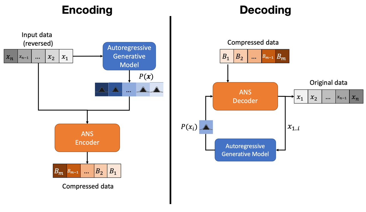
Figure 1: Entropy Encoding and Decoding with a Generative Autoregressive Model

From the left side of Figure 1, notice that we have to reverse the order of the input data to the ANS encoder (the autoregressive model receives the input in the usual parallel order though). This is needed because we need to decode the data in the ascending order for the autoregressive model to work (see decoding below). Next, notice that our ANS encoder requires both the (reversed) input data and the appropriate distributions for each symbol (i.e. each \(x_j\) component). Finally, the compressed data is output, which (hopefully) is shorter than the original input.

Decoding is shown on the right hand side of Figure 1. It's a bit more complicated because we must iteratively generate the distributions for each symbol. Starting by reversing the compressed data, we decode \(x_1\) since our model can unconditionally generate its distribution. This is the reason why we needed to reverse our input during encoding. Then, we generate \(x_2|x_1\) and so on for each \(x_i|x_{1,\ldots,i-1}\) until we've recovered the original data. Notice that this is quite inefficient since we have to call the model \(n\) times for each component of \(\bf x\).

I haven't tried this but it seems like something pretty reasonable to do (assuming you have a good model and I haven't made a serious logical error). The only problem with generative autoregressive models is that they are slow because you have to call them \(n\) times. Perhaps that's why no one is interested in this? In any case, the next method overcomes this problem.

2.2 Latent Variable Models

Latent variable models have a set of unobserved variables \(\bf z\) in addition to the observed ones \(\bf x\), giving us a likelihood function of \(P(\bf x|\bf z)\). We'll usually have a prior distribution \(P({\bf z})\) for \(\bf z\) (implicitly or explicitly), and depending on the model, we may or may not have access to a posterior distribution (more likely an estimate of it) as well: \(q(\bf z| \bf x)\).

The key idea with these models is that we need to encode the latent variables as well (or else we won't be able to generate the required distributions for \(\bf x\)). Let's take a look at Figure 2 to see how the encoding works.

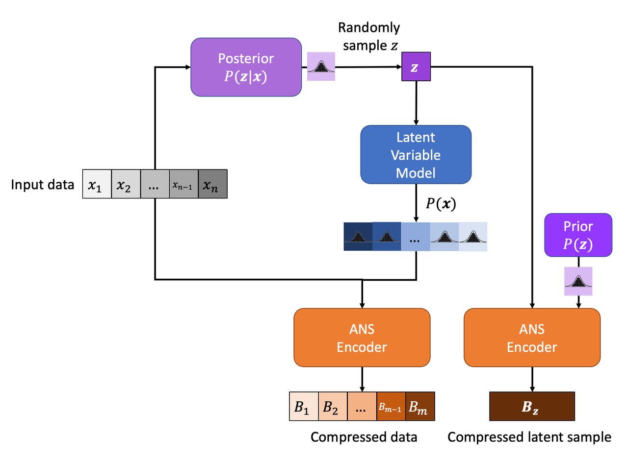
Figure 2: Entropy Encoding with a Latent Variable Model

Starting from the input data, we need to first generate some value for our latent variable \(\bf z\) so that we can use it with our model \(P(\bf x|\bf z)\). This can be obtained either by sampling the prior (or posterior if available), or really any other method that would generate an accurate distribution for \(\bf x\). Once we have \(\bf z\), we can run it through our model, get distributions for each \(x_i\) and encode the input data as usual. The one big difference is that we also have to encode our latent variables. The latent variables should be distributed according to our prior distribution (for most sensible models), so we can use it with the ANS coder to compress \(\bf z\). Notice that we cannot use the posterior here because we won't have access to \(\bf x\) at decompression time, therefore, would not be able to decompress \(\bf z\).

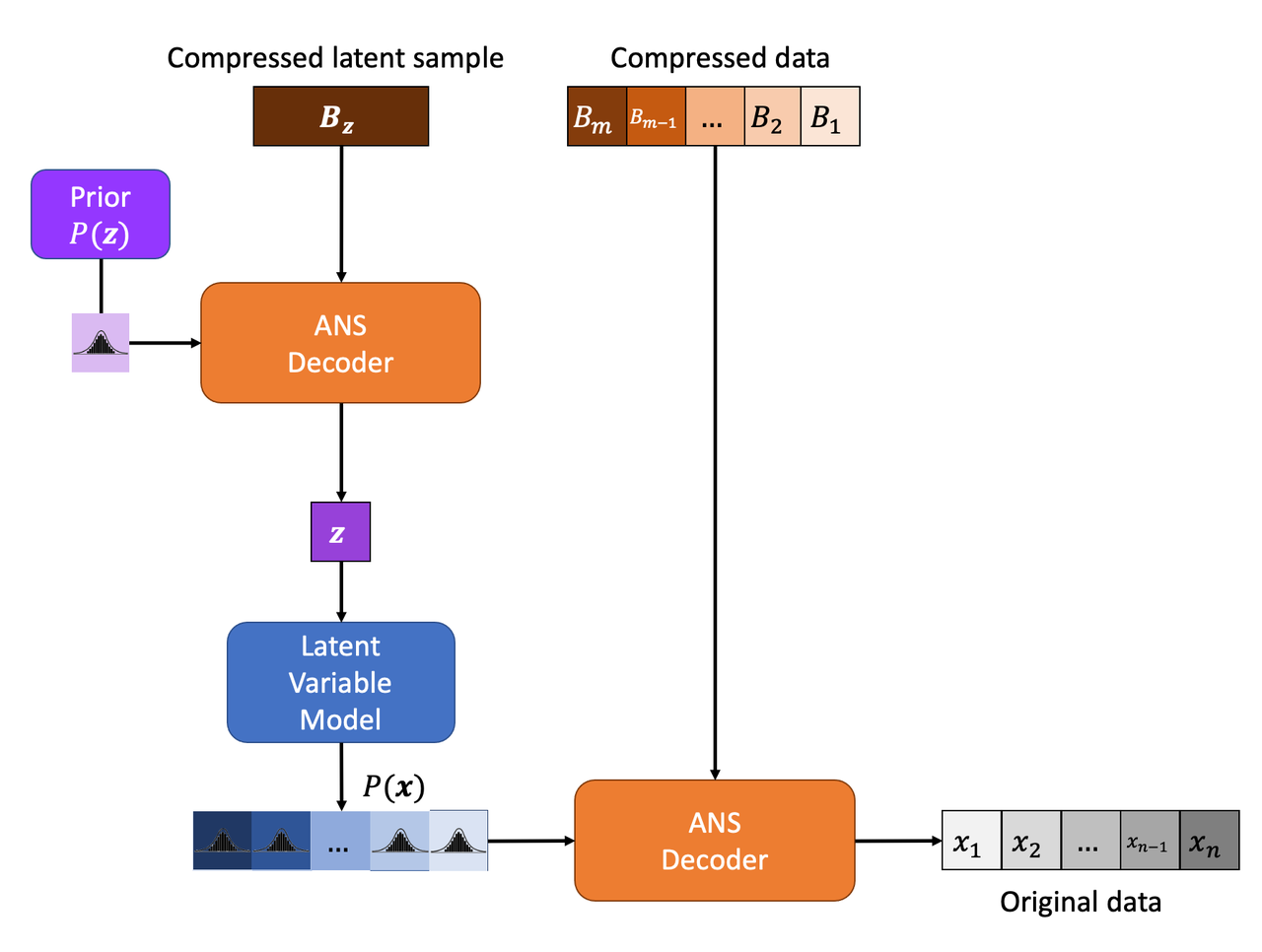
Figure 3: Entropy Decoding with a Latent Variable Model

Decoding is shown in Figure 3 and works basically as the reverse of encoding. The major thing to notice is that we have to do operations in a last-in-first-out order. That is, first decode \(\bf z\), use it to generate distributional outputs for the components of \(\bf x\), then use those outputs to decode the compressed data to recover our original message.

This is all relatively straight forward if you took time to think about it. There are some other issues as well around discretizing \(\bf z\) if it's continuous but we'll cover that below. The more interesting question is can we do better? The answer is a resounding "Yes!", and that's what this post is all about. By using a very clever trick you can get some "bits back" to improve your compression performance. Read on to find out more!

3 Bits-Back Coding

From the previous section, we know that we can encode and decode data using a latent variable model with relative ease. The big downside is that we're "wasting" space by encoding the latent variables. They're necessary to generate the distributions for our data, but otherwise are not directly encoding any signal. It turns out we can use a clever trick to recover some of this "waste".

Notice in Figure 2, we randomly sample from (an estimate of) the posterior distribution. In some sense, we're introducing new information from the random sample here that we must encode. Instead, why don't we utilize some of the existing bits we've encoded to get a "pseudo-random" sample 1 ? Figure 4 shows the encoding process in more detail.

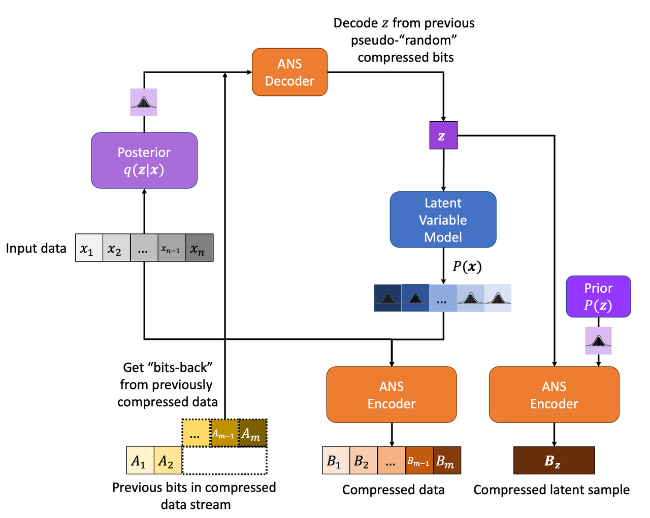
Figure 4: Bits-Back Encoding with a Latent Variable Model

The key difference here is that we're decoding the existing bitstream (from previous data that we've compressed) to generate a (pseudo-) random sample \(\bf z\) using the posterior distribution. This replaces the random sampling we did in Figure 2. Since the existing bitstream was encoded using a different distribution, the sample we decode should sort of random. The nice part about this trick is that we're still going to encode \(\bf z\) as usual so any bits we've popped off the bitstream to generate our pseudo-random sample, we get "back" (that is, aren't require to be on the bitstream anymore). This reduces the effective average size of encoding each datum + latent variables.

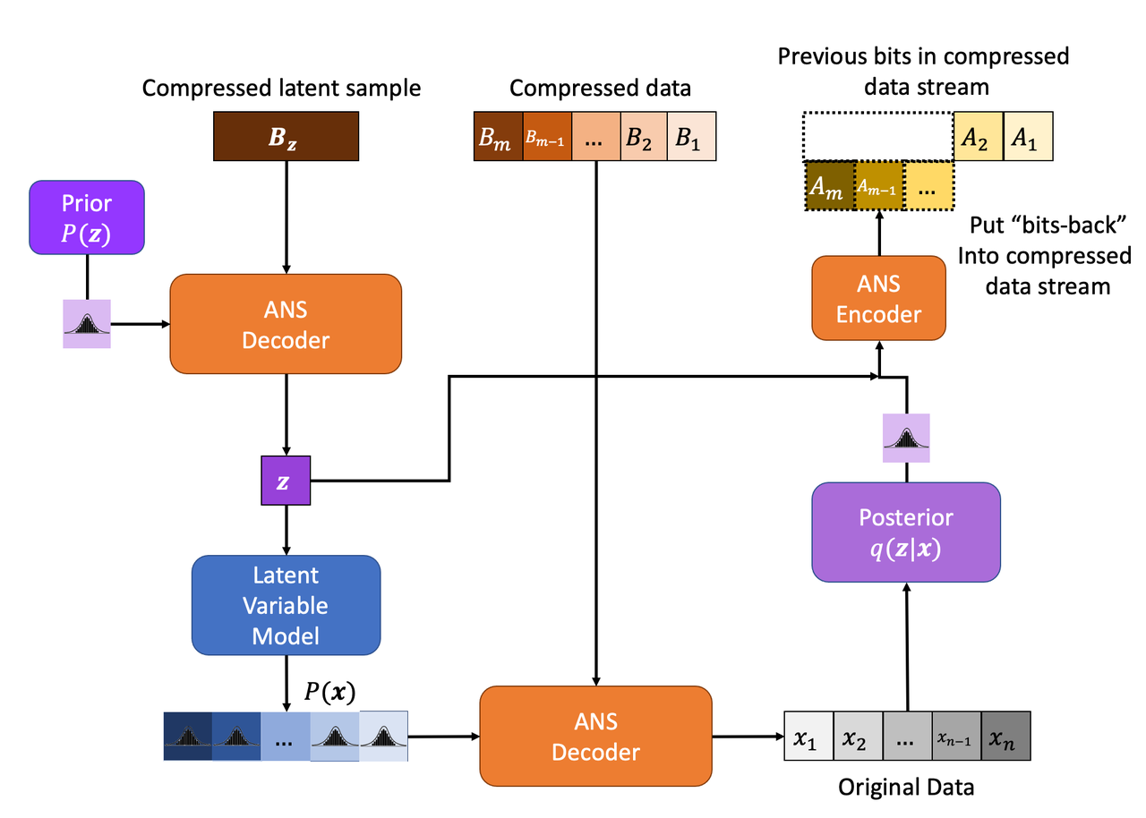
Figure 5: Bits-Back Decoding with a Latent Variable Model

Figure 5 shows decoding with Bits-Back. It is the same as latent variable decoding with the exception that we have to "put back" the bits we took off originally. Since our ANS encoding and decoding are lossless, the bits we put back should be exactly the bits we took off. The number of bits we removed/put back will be dependent on the posterior distribution and the bits that were originally there.

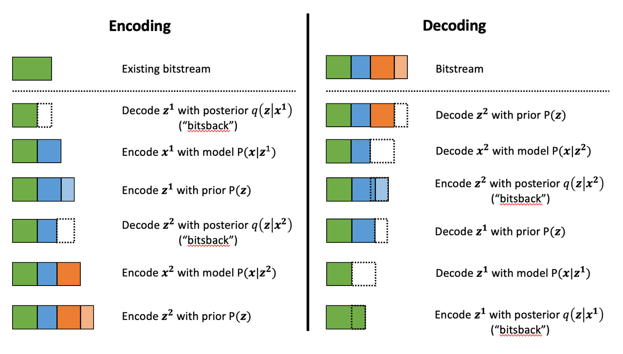
Figure 6: Visualization of Bitstream for Bits-Back Coding

To get a better sense of how it works, Figure 6 shows a visualization of encoding and decoding two data points. Colors represent the different data: green for existing bitstream, blue for \(\bf x^1\), and orange for \(\bf x^2\) (superscript represents data point index). The different shades represent either observed data \(\bf x\) or latent variable \(\bf z\).

From Figure 6, the first step in the process is to reduce the bitstream length by (pseudo-)randomly sampling \(\bf z\). This is followed by encoding \(\bf x\) and \(\bf z\) as usual. This process repeats for each additional datum. Even though we have to encode \(\bf z\), the effective size of the encoding is shorter because of the initial "bits back" we get each time. Decoding is the reverse operation of encoding: decode \(\bf z\) and \(\bf x\), put back the removed bits by utilizing the posterior distribution (which is conditional on the \(\bf x\) we just decoded). And this repeats until all data has been decoded.

4 Implementation Details

There were three main parts to my toy implementation: the ANS algorithm, a variational autoencoder, and the Bits-Back algorithm. Below are some details on each. You can find the code I used here on my Github.

ANS: The implementation I used was almost identical to the toy implementation I used from my previous post on ANS (which I wrote while travelling down the rabbit hole to understand the Bits-Back algorithm). That post has some details on the toy implementation that I used for it. These are notes for the incremental changes I made:

• I had to fix some slow parts of my implementation or else my experiments would have taken forever. For example, I was calculating the CDF in a slow way using native Python data structures. Switching to Numpy cusum fixed some of that. Additionally, I had to make sure that all my arrays were in Numpy objects and not slow native Python lists.

• As part of the algorithm, you have to calculate very big numbers that could exceed 64 bits (especially with an alphabet size of 256 and renormalization factor of 32). Python integers are great for this because they have arbitrary size. The only thing I had to be careful of was converting between my Numpy operations and Python integers. It was mostly just wrapping most expressions in the main calculation with int but took a bit to get it all sorted out.

• The code needed to be refactored a bit so it could be used in the Bits-Back algorithm. I refactored it to encode symbols incrementally instead of having the entire message available in the original implementation.

• I used 16 bits of quantization to model the distribution of the 256 pixel values and 32 bit renormalization.

Variational Autoencoder: I just used a vanilla VAE as the latent model since I was just experimenting on MNIST. In an effort to modernize, I started with the basic VAE Keras 2.0 example and added a few modifications:

• I added some ResNet identity blocks to beef up the representation power. Still not sure it really made much of a difference.

• Outputs of the decoder used my implementation of mixture of logistics to model the distributional outputs per pixel with 3 components. I wrote about it a bit in my PixelCNN post. I'm also wary about whether or not this actually made it better. The original paper [1] just used a Beta-Binomial distribution.

• I used 50 latent dimensions to match [1].

Bits-Back Algorithm: The Bits-Back algorithm is conceptually pretty simple but requires you to be a bit careful in a few areas. Here are some of the notable points:

• Since the quantization was always using equi-probable bins from a standard normal distribution, it made sense to cache the ranges for speeding it up.

• When quantizing the bins, you have to be careful at the edge bins which represent \(+\infty,-\infty\) and the quantized value for that bin obviously can't be infinity. I just used the next closest bin edge instead.

• Quantizing the continuous values of the latent variable distributions was a pain. For the case of quantizing a standard normal distribution (i.e., the prior), it was easy because, by construction, each bin is equi-probable. So the distribution is just uniform across however many buckets we are using (5-bits in my experiments).

• However, if you're trying to quantize a non-standard \(\bf z\) normal distributions using equi-probable bins from a standard normal distribution you have to be a bit more careful. Two big things to consider here:

  1. Ensure is that each bin has a non-zero probability or else when you're using it later to decode and gets bits back, you might actually end up seeing a zero probability symbol, which will break things. Specifically, you want each bucket to have at least probability \(\frac{1}{2^{n}}\).

  2. You want the quantized distribution to best match the original non-quantized one but with the constraint that we have some mass in each bin. Here's the algorithm I used:

     • First, define the number of symbols in your alphabet \(m\) (i.e., number of bins); I used \(m=5\).

     • Sample \(2^n - 2^m\) for \((n=16, m=5)\) equi-probable-spaced values per variable from the original \(\bf z\) distributions using the inverse CDF function from SciPy. This guarantees you get good representation from the entire distribution.

     • From those sampled values, make a frequency histogram where the buckets correspond to the \(m\) equi-probable buckets. This is essentially the probability distribution in frequency form.

     • Add 1 to each of the histogram buckets to guarantee a non-zero probability mass (see point 1 above).

     • This histogram serves as the probability distribution used by rANS to decode the required values. And because of the way rANS algorithm works, it uses a frequency distribution so I could just pass it directly to the compressor.

     I'm not sure if there's a better way to do it but it seemed work well enough.

• Encoding/decoding the \(x\) pixel values was much easier because they are already discretized as 256 pixel values. It's still a bit slow though since I just loop through each pixel value and encode it sequentially.

• The only tricky part for the pixel values was that I had to translate the probability distribution (real numbers) over discrete pixels into a frequency distribution (integers). That is for each pixel, we have discrete distribution over the 256 values but each value has a real number that represents its probability. So we need to convert it to a frequency distribution in order to pass it to ANS.

• The sum of the frequency distribution also needs to sum to \(2^{n}\). Additionally, I wanted to ensure that no bin had zero probability (same issue as above). To pull this off, I just multiplied each bin's probability by \(2^{n}\), added one to each bin, then calculate any excess I have beyond \(2^{n}\) and shave it off the largest frequency bin. This is obviously not an optimal way to do it but it probably doesn't affect too much.

• Again, I had to be careful not to implicitly convert some of the integer values to floats. So in some places, I do some explicit casting of astype(np.uint64) so the values don't get all mixed up when I send them into ANS.

5 Experiments

My compression results for MNIST (regular, non-binarized) are shown in Table 1. My implementation can achieve 1.5264 bits/pixel (i.e. on average a pixel uses 1.53 bits to represent it) vs. other implementations of 1.4 or less. That's not half bad (better than my original implementation which had a bug where I got closer to 1.9 bits/pixel)! I was at least able to beat gzip, which says something. It still feels kind of far from [1] at 1.41, but it feels like I got the main theoretical parts worked out.

Interestingly [1] was using a simpler model (a single feed-forward layer for each of the encoder/decoder) with a Beta-Binomial output distribution for each pixel. This is obviously simpler than my complex ResNet/multi-logistic method. It's possible that I'm just not able to get a good fit with my VAE model. If you take a look in the notebook you'll see that the generated digits I can make with the decoder look pretty bad. So this is probably at least part of the reason why I was unable to achieve good results.

The second reason is that I suspect my quantization isn't so great. As mentioned above, I did so funky rounding to ensure no zero-probability buckets, as well as an awkward way to discretize the latent variables and data. I suspect there are some differences from [1]'s implementation (which is open source by the way) but I didn't spend too much time trying to diagnose the differences.

In any case, at least my implementation is able to correctly encode and decode and somewhat approach the proper implementations. As a toy implementation, I will make the bold assertion that I coded it in a way that's a bit more clear than [1]'s implementation (and has this handy write up) so maybe it's better for educational purposes? I'll let you be the judge of that.

6 Conclusion

So there you have it, a method for lossless compression using ML! This mix of discrete problems (e.g. compression) and ML is an incredibly interesting direction. If I get some time (and who knows when that will be), I'm definitely going to be looking into some more of these topics. But on this lossless compression topic, I'm probably done for now. There's another topic that I've been excited about recently and have already started to go down that rabbit hole, so expect one (probably more) posts on that subject. Hope everyone is staying safe!

7 References

• Previous posts: Variational Autoencoders, Lossless Compression with Asymmetric Numeral Systems, Expectation Maximization Algorithm

• My implementation on Github: notebooks

• [1] "Practical Lossless Compression with Latent Variables using Bits Back Coding", Townsend, Bird, Barber, ICLR 2019.

• [2] "Bit-Swap: Recursive Bits-Back Coding for Lossless Compression with Hierarchical Latent Variables", Kingma, Abbeel, Ho, ICML 2019

1

I'll be using this term "pseudo-random" to describe this faux random sampling process. I know it's probably not accurate to even call it pseudo-random, but I'm using it colloquially to mean not truly random.