Sampling from a Normal Distribution

One of the most common probability distributions is the normal (or Gaussian) distribution. Many natural phenomena can be modeled using a normal distribution. It's also of great importance due to its relation to the Central Limit Theorem.

In this post, we'll be reviewing the normal distribution and looking at how to draw samples from it using two methods. The first method using the central limit theorem, and the second method using the Box-Muller transform. As usual, some brief coverage of the mathematics and code will be included to help drive intuition.

Background¶

Normal Distribution¶

Let's start off first by covering some basics. A normal distribution (also known as a Gaussian distribution) $N \sim (\mu, \sigma)$ has probability density function (PDF) and cumulative density function (CDF) shown here parameterized by its mean ($\mu$) and standard deviation ($\sigma$) ^[1]:

$$ f_N(x) = \frac{1}{\sigma \sqrt{2\pi}}e^{-\frac{(x-\mu)^2}{2\sigma^2}} \tag{1}$$$$ F_N(x) = \int_{-\infty}^{x}f_N(t) dt \tag{2}$$

The CDF doesn't have a nice closed form, so we'll just represent it here using the definition of CDF in terms of its PDF. We can graph the PDF and CDF (images from Wikipedia) using various values of the two parameters:

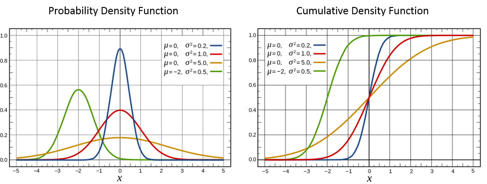
The normal distribution is sometimes colloquially known as the "bell curve" because of a it's symmetric hump. A very common thing to do with a probability distribution is to sample from it. In other words, we want to randomly generate numbers (i.e. $x$ values) such that the values of $x$ are in proportion to the PDF. So for the standard normal distribution, $N \sim (0, 1) $ (the red curve in the picture above), most of the values would fall close to somewhere around $x=0$. In fact, 68% will fall within $[-1, 1]$, 95% will fall within $[-2,2]$ and 99.7% will fall within $[-3,3]$. This corresponds to $\sigma, 2\sigma, 3\sigma$ from the mean, see this article for more details.

Central Limit Theorem¶

The central limit theorem (CLT) is quite a surprising result relating the sample average of $n$ independent and identically distributed (i.i.d.) random variables and a normal distribution. To state it more precisely:

Let ${X_1, X_2, \ldots, X_n}$ be $n$ i.i.d. random variables with $E(X_i)=\mu$ and $Var(X_i)=\sigma^2$ and let $S_n = \frac{X_1 + X_2 + \ldots + X_n}{n}$ be the sample average. Then $S_n$ approximates a normal distribution with mean of $\mu$ and variance of $\frac{\sigma^2}{n}$ for large $n$ (i.e. $S_n \approx N(\mu, \frac{\sigma^2}{n})$).

The surprising result is that $X_n$ can be any distribution. It isn't restricted to just normal distributions. We can also define the standard normal distribution in terms of $S_n$ by shifting and scaling it:

$$ N(0,1) \approx \frac{S_n - \mu}{\frac{\sigma}{\sqrt{n}}} = \frac{\sqrt{n}(S_n - \mu)}{\sigma} \tag{3} $$

Comparing Distributions¶

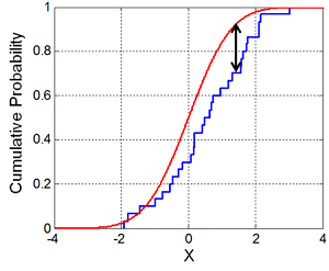
Since our goal is to implement sampling from a normal distribution, it would be nice to know if we actually did it correctly! One common way to test if two arbitrary distributions are the same is to use the Kolmogorov–Smirnov test. In the basic form, we can compare a sample of points with a reference distribution to find their similarity.

The basic idea of the test is to first sort the points in the sample and the compute the empirical CDF. Next, find the largest absolute difference between any point in the empirical CDF and the theoretical reference distribution. If the two are the same, this difference should be very small. If it's large then we can be confident that the distribution is different. Further, this difference follows a certain distribution, which allows us to test our null hypothesis of whether our samples were drawn from the reference distribution.
The following figure (from Wikipedia) shows this more clearly:

Fortunately, we don't have to implement this ourselves. A package is available in scipy.stats. Let's play around with it a bit to see how it works.

Using $N(0,1)$ as our reference distribution, the KS test has a large value and a negligible p-value when comparing to a uniform distribution $U(0,1)$ ($KS=0.5$). The normal distribution with a wider base $N(0, 2)$ ($KS=0.1673$) also has a negligible p-value. However, when we compare samples from the identical distribution $N(0,1)$, we get a relatively small value ($KS=0.0104$) for the test statistic and a large p-value, indicating we don't have sufficient evidence to reject the null hypothesis (that our two distributions are the same).

Sampling using the Central Limit Theorem¶

Now let's try to use the Central Limit Theorem to sample from $N(0,1)$. First let's define our i.i.d. variable $X_n$ to have a Bernoulli distribution with $p=0.5$, which we can intuitively think of tossing an unbiased coin:

$$ P(X_n=k) = \begin{cases} p=0.5 & \text{if }k=1, \\[6pt] 1-p = 0.5 & \text {if }k=0.\end{cases} \tag{4} $$

Recall, the Bernoulli distribution is closely relates to the Binomial distribution denoted by $B(n, p)$ by $Bernoulli(p) = B(n=1, p)$ . The Binomial distribution can intuitively be thought of as counting the number of heads in $n$ tosses of a coin (i.e. Bernoulli trials). If $n=1$, it reduces to a Bernoulli distribution (or single coin toss).

Let's now define our sample average for $n$ tosses of our unbiased coin:

$$ S_n = \frac{X_1 + X_2 + \ldots + X_n}{n} = \frac{B(n, p=0.5)}{n} $$

We know that a Bernoulli distribution has $\mu=\frac{1}{2}$ (we expect half our tosses to be heads), and $\sigma^2=p(1-p)=0.25$.

Shifting and scaling^[2] this to get our standard normal distribution using Equation 3, we get:

\begin{align} N(0,1) &\approx \frac{\sqrt{n}(S_n - \mu)}{\sigma} \\ &= \frac{\sqrt{n}(\frac{X_1 + X_2 + \ldots + X_n}{n} - 0.5)}{\sqrt{0.25}} \\ &= 2\sqrt{n}(\frac{X_1 + X_2 + \ldots + X_n}{n} - 0.5) \tag{5} \end{align}

Theoretically, this should give us an equation to roughly simulate a standard normal distribution. Let's try it!

Our KS score is somewhat close to $0$ with a p-value that suggests we can't reject our null hypothesis. Graphing our implementation of $N(0,1)$ with the reference one shows that we have the roughly the right shape. No doubt by setting larger $N$ (for both the number of Bernoulli trials and the number of samples drawn), we would get something much closer.

One large downside of our CLT implementation is that it's slow. While the wall clock time of drawing $10000$ samples using the numpy library is unnoticeable, it takes roughly ten seconds on my machine with the parameters above using our CLT implementation, quite a big difference. In the next section, we'll see a much more efficient implementation that uses a "trick" to transform a pair of independent uniform random variables to a pair of independent normal random variables.

Sampling using the Box-Muller Transform¶

The Box-Muller transform is a neat little "trick" that allows us to sample from a pair of normally distributed variables using a source of only uniformly distributed variables. The transform is actually pretty simple to compute. Given two independent uniformly distributed random variables $U_1, U_2$ on the interval $(0,1)$, we define two new random variables, $R$ and $\Theta$, that intuitively representing polar coordinates as such:

\begin{align} R &= \sqrt{-2lnU_1} \tag{6}\\ \Theta &= 2\pi U_2 \tag{7} \end{align}

Now using the standard transformation from polar coordinates $R, \Theta$ to Cartesian ones $X, Y$, we claim that $X$ and $Y$ are independent standard normally distributed random variables:

\begin{align} X &= Rcos\Theta &= \sqrt{-2lnU_1}cos(2\pi U_2) \tag{8}\\ Y &= Rsin\Theta &= \sqrt{-2lnU_1}sin(2\pi U_2) \tag{9} \end{align}

Let's take a look at the proof to gain some intuition on how this works.

Proof¶

Starting with $U_1, U_2$, let's see what kind of distributions we have for $R, \Theta$. From Equation 7, it should be clear that $\Theta$ is also uniformly distributed since it's just multiplying by a constant ($2\pi$), but let's go through the motions to explicitly see that. From the CDF of $\Theta$:

\begin{align} P(\Theta \leq \theta) &= P(2\pi U_2 \leq \theta) \\ &= P(U_2 \leq \frac{\theta}{2\pi}) \\ \Theta &\sim Uniform(0, 2\pi) \tag{10} \end{align}

So we have our first result that $\Theta$ is uniformly distributed on $(0, 2\pi)$ (as we would expect). Using a more explicit method, we can find the distribution of $R$. From Equation 7, we know that the mapping from $U_1$ to $R$ is one-to-one, which we'll call $g$ (i.e. $R=g(U_1)$). So if we're trying to find the probability of R over $(r_1, r_2)$ (by integrating its PDF), there is some equivalent range over $(g^{-1}(r_1), g^{-1}(r_2))$ where we can integrate over the PDF of $U_1$. Let's see how this works ^[3]:

\begin{align} P(r_1 \leq R \leq r_2) &= \int_{g^{-1}(r_2)}^{g^{-1}(r_1)} f_{U_1}(s) ds && \text{since } g(x) \text{ is strictly decreasing}\\ &= -\int_{g^{-1}(r_1)}^{g^{-1}(r_2)} ds && \text{since }f_{U_1}(u)=1 \\ &= -\int_{r_1}^{r_2} -t e^{\frac{-t^2}{2}} dt && \text{change variables } t=\sqrt{-2\ln s}\tag{11} \\ f_R(r) &= r e^{\frac{-r^2}{2}} \tag{12} \end{align}

giving us the PDF for $R$, $f_R(r)$^[4]. It should also be clear that $R$ and $\Theta$ are independent because $U_1$ and $U_2$ are independent.

Now that we have the distributions for both $R$ and $\Theta$, let's label Equation 8 and 9 as $X=g_x(R, \Theta)$ and $Y=g_y(R, \Theta)$, respectively. Now we can apply the same procedure as above using variable substitution (for multiple variables) to derive the joint distribution of $X$ and $Y$ (we'll represent the area in the transformed space by $A$^[5]):

\begin{align} P(x_1 &\leq X \leq x_2, y_1 \leq Y \leq y_2) \\ &= \int \int_A f_{R,\Theta}(u, v) du dv \\ &= \int \int_A f_{R}(u)f_{\Theta}(v) du dv && \text{since } R \text{ and } \Theta \text{ are independent} \\ &= \int \int_A ue^{\frac{-u^2}{2}}\frac{1}{2\pi} du dv \tag{13} \end{align}

At this point, we should remember that if $p=ucos(v), q=usin(v)$, then solving for $u,v$ results in $u=\sqrt{q^2+p^2}, v=arctan(\frac{q}{p})$. Also, substitution for multiple variables means that $du dv = |det(\frac{\partial(u,v)}{\partial(p, q)})| dp dq$, plugging our expressions for $u$ and $v$ in:

\begin{align} du dv &= |det(\frac{\partial(u,v)}{\partial(p, q)})| dp dq \\ &= \left | \begin{array}{cc} \frac{\partial u}{\partial p} & \frac{\partial u}{\partial q} \\ \frac{\partial v}{\partial p} & \frac{\partial v}{\partial q} \end{array} \right | dpdq \\ &= \left | \begin{array}{cc} \frac{\partial \sqrt{q^2+p^2}}{\partial p} & \frac{\partial \sqrt{q^2+p^2}}{\partial q} \\ \frac{\partial arctan(\frac{q}{p})}{\partial p} & \frac{\partial arctan(\frac{q}{p})}{\partial q} \end{array} \right | dpdq \\ &= \left | \begin{array}{cc} \frac{p}{\sqrt{p^2+q^2}} & \frac{q}{\sqrt{p^2+q^2}} \\ \frac{-q}{p^2(1+(\frac{q}{p})^2)} & \frac{1}{p(1+(\frac{q}{p})^2)} \end{array} \right | dpdq \\ &= \frac{1}{\sqrt{p^2 + q^2}} dpdq \tag{14} \end{align}

Using the result from Equation 14 into Equation 13, we get:

\begin{align} P(&x_1 \leq X \leq x_2, y_1 \leq Y \leq y_2) && \text{change variables} \\ &= \int_{x_1}^{x_2} \int_{y_1}^{y_2} \frac{\sqrt{p^2 + q^2}}{2\pi}\cdot e^{\frac{-(p^2 + q^2)}{2}} \cdot \frac{1}{\sqrt{p^2 + q^2}} dp dq && p=ucos(v) \\ & && q=usin(v) \\ &= \int_{x_1}^{x_2} \underbrace{\frac{1}{\sqrt{2\pi}} e^{\frac{-p^2}{2}}}_{f_X(x)} dp \int_{y_1}^{y_2} \underbrace{\frac{1}{\sqrt{2\pi}} e^{\frac{-q^2}{2}}}_{f_Y(y)} dq \tag{15} \end{align}

Equation 15 shows that $X$ and $Y$ are independent each with PDF matching our standard normal distribution $N(0,1)$ as required.

Implementing Box-Muller Transform¶

The implementation is a relatively straight forward application of Equation 8 and 9:

As we can see, our Box-Muller method of sampling from $ N(0,1) $ generates quite good results. Our KS test statistic is quite small along with a large p-value (so we can't reject our null hypothesis). Similarly, the graph shows the expected shape matching our reference distribution. The one big advantage this method has though is that it's quite fast. There's no noticeable lag when generating (N=10000) samples.

Conclusion¶

Generating pseudo-random numbers according to various probability distributions has many applications, for example, in Markov Chain Monte Carlo (MCMC) techniques. In this post, we looked at one of the most fundamental distributions: the standard normal distribution. Our first method uses a result directly from the central limit theorem which results in an inefficient implementation. However with a bit of grit and calculus, we were able to show that the Box-Muller transform provides a much more elegant solution to sampling from a standard normal distribution leading us to an efficient implementation. Hopefully this sheds some light on how to sample a normal distribution.

References and Further Reading¶

• Wikipedia: Normal Distribution, Box-Muller Transform, Central Limit Theorem, Substitution for multiple variables, Determinant of 2x2 matrices, Jacobian matrix and determinant
• Stack Exchange: How to sample from a normal distribution with known mean and variance using a conventional programming language?, Proof of Box-Muller method
• Transformations of Random Variables (University of Alabama Huntsville)
• Change of Variables (Paul's Online Math Notes)
• Simple Sampling of Gaussians (Jonathan Goodman, NYU)

Notes¶

List of Notes: ¹, ², ³, ⁴, ⁵