An Introduction to Stochastic Calculus

2.1 Probability Spaces & Random Variables

(Note: Skip this part if you're already familiar with the measure theoretic definition of probability.)

We're going to dive into the measure theoretic definition of probability, attempting to give some intuition while still maintaining some level of rigour. First, let's examine the definition of a probability space \((\Omega, {\mathcal {F}}, P)\). This is the same basic idea you learn in a first probability course except with fancier math.

\(\Omega\) is the sample space, which defines the set of all possible outcomes of an experiment. In finite sample spaces, any subset of the sample space is called an event. Another way to think about events is any grouping of objects you would want to measure the probability on (e.g., individual elements of \(\Omega\), unions of elements, or even the empty set).

However, this type of reasoning breaks down when we have certain types of infinite sample spaces (e.g., real line). For this, we need to define an event more precisely with an event space \(\mathcal{F} \subseteq 2^{\Omega}\) (\(2^{\Omega}\) denotes the power set) using a construction called a \(\sigma\)-algebra ("sigma algebra"):

Let \(\Omega\) be a non-empty set, and let \(\mathcal{F}\) be a collection of subsets of \(\Omega\). We say that \(\mathcal{F}\) is a \(\sigma\)-algebra: if:

1. The empty set belongs to \(\mathcal{F}\).

2. Whenever a set \(A\) belongs to \(\mathcal{F}\), its compliment \(A^c\) also belongs to \(\mathcal{F}\) (closed under complement).

3. Whenever a sequence of sets \(A_1, A_2, \ldots\) belongs to \(\mathcal{F}\), their union \(\cup_{n=1}^{\infty} A_n\) also belongs to \(\mathcal{F}\) (closed under countable unions -- implies closed under countable intersection).

The elements of a \(\sigma\)-algebra are called measurable sets, and the pair \((\Omega, \mathcal{F})\) define a measurable space.

Thus, we wish our event space \(\mathcal{F}\) to be a \(\sigma\)-algebra and when combined with \(\Omega\), define a measurable space. This sounds complicated but it basically guarantees that the subsets of \(\Omega\) that we use for events have all the nice properties we would expect from probabilities.

Intuitively, measurable spaces help makes the notion of "size" or "volume" precise by defining the "chunks" of "volume". Using a physical analogy, you want to make sure that no matter how you combine non-overlapping "chunks" (i.e., unions of disjoint sets), you end up with a consistent measure of "volume". Again, this is only really needed with infinite (non-countable) sets. For finite event spaces, we can usually just use the power set \(2^{\Omega}\) as the event space, which has all these properties above.

And this brings us to the last part of probability spaces:

A probability measure \(P\) on an event space \(\mathcal{F}\) is a function that:

1. Maps events to the unit interval \([0, 1]\),

2. Returns \(0\) for the empty set and \(1\) for the entire space,

3. Satisfies countable additivity for all countable collections of events \(\{E_i\}\) of pairwise disjoint sets:

   \begin{equation*} P(\cup_{i\in I} E_i) = \Sigma_{i\in I} P(E_i) \tag{2.1} \end{equation*}

These properties should look familiar as they are the three basic ones axioms everyone learns when first studying probability. The only difference is that we're formalizing them, particularly the last one where we may not have seen it with respect to infinite collections of events.

Going back to the "volume" analogy above, the probability measure maps the "chunks" of our "volume" to \([0,1]\) (or non-negative real numbers for general measures) but in a consistent way. Due to the way we've defined event spaces as \(\sigma\)-algebra's along with the third condition from Equation 2.1, we get a consistent measurement of "volume" regardless of how we combine the "chunks". Again, for finite sample spaces, it's not too hard to imagine this function but for continuous sample spaces, it gets more complicated. All this is essentially to define a rigorous construction that matches our intuition of basic probability with samples spaces, events, and probabilities.

Finally, for a given probability space \((\Omega, {\mathcal {F}}, P)\):

A random variable \(X\) 1 is a measurable function \(X:\Omega \rightarrow E \subseteq \mathbb{R}\) where:

1. \(X\) must part of a measurable space, \((E, \mathcal{S})\) (recall: \(\mathcal{S}\) defines a \(\sigma\)-algebra on the set \(E\)). For finite or countably infinite values of \(X\), we generally use the powerset of \(E\). Otherwise, we will typically use the Borel set for uncountably infinite sets (e.g., the real numbers).

2. For all \(s \in \mathcal{S}\), the pre-image of \(s\) under \(X\) is in \(\mathcal{F}\). More precisely:

   \begin{equation*} \{X \in \mathcal{s}\} \in \mathcal{F} := \{\omega \in \Omega | X(\omega) \in s\} \in \mathcal{F} \tag{2.2} \end{equation*}

We use random variables to map outcomes from our event space to the real line (e.g., a RV for a coin flip where heads maps to 1 and tails maps to 0). However, the mapping must also have the same consistency as we defined above. So this definition basically ensures that every value that \(X\) can take on (which must be measurable) has a mapping to one of the measurable events in our original event space \(\mathcal{F}\). We use the notation \(\sigma(X)\) to denote the collection of all subsets of Equation 2.2, which form the \(\sigma\)-algebra implied by the random variable \(X\).

If we didn't have this condition then either: (a) we couldn't properly measure \(X\)'s "volume" because our "chunks" would be inconsistent (constraint 1), or (b) we wouldn't be able to map it back to "chunks" in our original probability space and apply \(P\) to evaluate the random variable's probability. If this all seems a little abstract, it is, but that's what we need when we're dealing with uncountable infinities. Again, for the finite cases, all of these properties are trivially met.

Using the probability measure \(P\), one can calculate the probability of \(X \in \mathcal{S}\) using Equation 2.2:

where \(s \subseteq \mathcal{S}\) and \(f\) is the corresponding event in \(\mathcal{F}\). We can take \(s = \{x\}\) to evaluate the random variable at a particular value. Equation 2.3 basically says that we map backwards from a set of real numbers (\(s\)) to a set of values in the sample space (i.e., an event given by Equation 2.2) using the inverse of function \(X\). From the event in our event space \(f \subseteq \mathcal{F}\), which is guaranteed to exist because of property (2), we know how to compute the probability using \(P\).

So a random variable then allows us to map to real numbers from our original sample space (\(\Omega\)). Often times our sample space has no concept of numbers (e.g., heads or tails) but random variables allow us to assign real numbers to those events to calculate things like expected values and variances.

For many applications of probability, understanding the above is overkill. Most practitioners of probability can get away with the "first stage" (see box below) of learning probability. However specifically for stochastic calculus, the above helps us learn it beyond a superficial level (arguably) because we quickly get into situations where we need to understand the mathematical rigour needed for uncountable infinities.

2.2 Stochastic Processes

Here's the formal definition of a stochastic process from [2]:

Suppose that \((\Omega,\mathcal{F},P)\) is a probability space, and that \(T \subset \mathbb{R}\) is of infinite cardinality. Suppose further that for each \(t \in T\), there is a random variable \(X_t: \Omega \rightarrow \mathbb{R}\) defined on \((\Omega,\mathcal{F},P)\). The function \(X: T \times \Omega \rightarrow \mathbb{R}\) defined by \(X(t, \omega) = X_t(\omega)\) is called a stochastic process with indexing set \(T\), and is written \(X = \{X_t, t \in T\}\).

That's a mouthful! Let's break this down and interpret the definition more intuitively. We've already seen probability spaces and random variables in the previous subsection. The first layer of a stochastic process is that we have a bunch of random variables that are indexed by some set \(T\). Usually \(T\) is some total ordered sequence such as a subset of the real line (e.g., \((0, \infty)\)) or natural numbers (e.g., \(0, 1, 2, 3 \ldots\)), which intuitively correspond to continuous and discrete time.

Next, we turn to the probability space on which each random variable is defined on \((\Omega,\mathcal{F},P)\). The key thing to note is that the elements of the sample space \(\omega \in \Omega\) are infinite sets that correspond to experiments performed at each index in \(T\). (Note: by definition it's infinite because otherwise it would just be a random vector.) For example, flipping a coin at every (discrete) time from \(0\) to \(\infty\), would define a specific infinite sequence of heads and tails \(\omega = \{H, T, H, H, H, T, \ldots\}\). So each random variable \(X_t\) can depend on the entire sequence of the outcome of this infinite "experiment". That is, \(X_t\) is a mapping from outcomes of our infinite experiment to (a subset of) the real numbers: \(X_t: \Omega \rightarrow E \subseteq \mathbb{R}\). It's important to note that in this general definition we have no explicit concept of time, so we can depend on the "future". To include our usual concept of time, we need an additional concept (see adapted processes below).

Finally, instead of viewing the stochastic process as a collection of random variables indexed by time, we could look at it as a function of both time and the sample space i.e., \(X(t, \omega) = X_t(\omega)\). For a given outcome of an experiment \(\omega_0\), the deterministic function generated as \(X(t, \omega=\omega_0)\) is called the sample function. However, mostly we like to think of it as having a random variable at each time step indicated by this notation: \(X = \{X_t, t \in T\}\). We sometimes use the notation \(X(t)\) to refer to the random variable at time \(t\) or the stochastic process itself.

Stochastic processes can be classified by the nature of the values the random variables take and/or the nature of the index set:

• Discrete and Continuous Value Processes: \(X(t)\) is discrete if at all "times" \(X(t)\) takes on values in a countable set (i.e., can be mapped to a subset of the natural numbers); otherwise \(X(t)\) is continuous.

• Discrete and Continuous Time Processes: \(X(t)\) is discrete time process if the index set is countable (i.e., can be mapped to a subset of the natural numbers), otherwise it is a continuous time process.

Generally continuous time processes are harder to analyze and will be the focus of later sections. The next two discrete time examples give some intuition about how to match the formal definition to concrete stochastic processes.

Example 3: One Dimensional Symmetric Random Walk

A simple one dimensional symmetric random walk is a discrete value, discrete time stochastic process. An easy way to think of it is: starting at 0, at each time step, flip a fair coin and move up (+1) if heads, otherwise move down (-1).

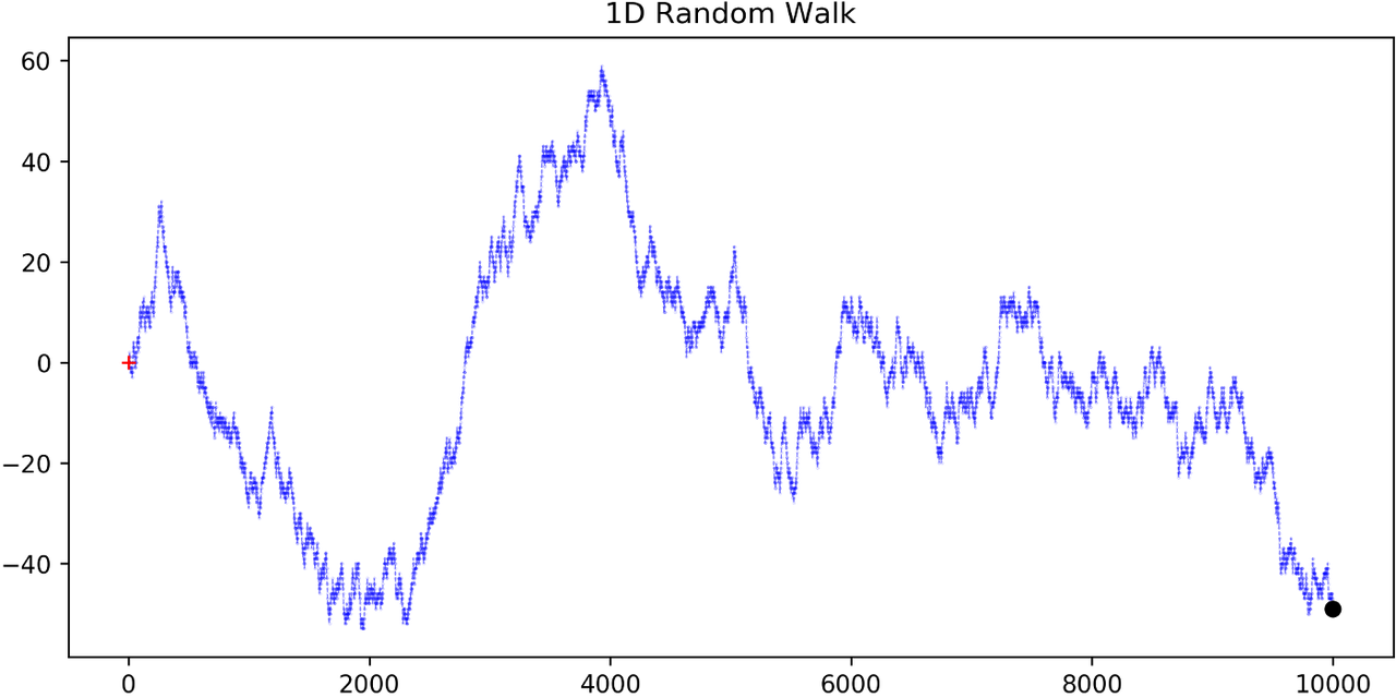
Figure 1: 1D Symmetric Random Walk (source)

This can be defined in terms of the Bernoulli process \(X_t\) from Example 2 with \(p=0.5\) (with the same probability space):

\begin{equation*} S_t(\omega) = \sum_{i=1}^t X_t \tag{2.8} \end{equation*}

Notice that the random variable at each time step depends on all the "coin flips" \(X_t\) that came before it, which is in contrast to just the current "coin flip" for the Bernoulli process.

Another couple of results that we'll use later. The first is that the increments between any two given non-overlapping pairs of integers \(0 = k_0 < k_1 < k_2 < \ldots < k_m\) are independent. That is, \((S_{k_1} - S_{k_0}), (S_{k_2} - S_{k_1}), (S_{k_3} - S_{k_2}), \ldots, (S_{k_m} - S_{k_{m-1}})\) are independent. We can see this because for any combination of pairs of these differences, we see that the independent \(X_t\) variables don't overlap, so the sum of them must also be independent.

Moreover, the expected value and variance of the differences is given by:

\begin{align*} E[S_{k_{i+1}} - S_{k_i}] &= E[\sum_{j=k_i + 1}^{k_{i+1}} X_j] \\ &= \sum_{j=k_i + 1}^{k_{i+1}} E[X_j] \\ &= 0 \\ Var[S_{k_{i+1}} - S_{k_i}] &= Var[\sum_{j=k_i + 1}^{k_{i+1}} X_j] \\ &= \sum_{j=k_i + 1}^{k_{i+1}} Var[X_j] && X_j \text{ independent}\\ &= \sum_{j=k_i + 1}^{k_{i+1}} 1 && Var[X_j] = E[X_j^2] = 1 \\ &= k_{i+1} - k_i \\ \tag{2.9} \end{align*}

Which means that the variance of the symmetric random walk accumulates at a rate of one per unit time. So if you take \(l\) steps from the current position, you can expect a variance of \(l\). We'll see this pattern when we discuss the extension to continuous time.

2.3 Adapted Processes

Notice that in the previous section, our definition of stochastic process included a random variable \(X_t: \Omega \rightarrow E \subseteq \mathbb{R}\) where each \(\omega \in \Omega\) is an infinite sequence representing a given outcome for the infinitely long experiment. This implicitly means that at "time" \(t\), we could depend on the "future" because we are allowed to depend on any tosses, including those greater than \(t\). In many applications, we do want to interpret \(t\) as time so we wish to restrict our definition of stochastic processes.

An adapted stochastic process is one that cannot "see into the future". Informally, it means that for any \(X_t\), you can determine it's value by only seeing the outcome of the experiment up to time \(t\) (i.e., \(\omega_1\omega_2\ldots\omega_t\) only).

To define this more formally, we need to introduce a few technical definitions. We've already seen the definition of the \(\sigma\)-algebra \(\sigma(X)\) implied by the random variable \(X\) in a previous subsections. Suppose we have a subset of our event space \(\mathcal{G}\), we say that \(X\) is \(\mathcal{G}\)-measurable if every set in \(\sigma(X) \subseteq \mathcal{G}\). That is, we can use \(\mathcal{G}\) to "measure" anything we do with \(X\).

Using this idea, we define the concept of a filtration on our event space \(\mathcal{F}\) and our index set \(T\):

A filtration \(\mathbb{F}\) is a ordered collection of subsets \(\mathbb{F} := (\mathcal{F_t})_{t\in T}\) where \(\mathcal{F_t}\) is a sub-\(\sigma\)-algebra of \(\mathcal{F}\) and \(\mathcal{F_{t_1}} \subseteq \mathcal{F_{t_2}}\) for all \(t_1 \leq t_2\).

To break this down, we're basically saying that our event space \(\mathcal{F}\) can be broken down into logical "sub event spaces" \(\mathcal{F_t}\) such that each one is a superset of the next one. This is precisely what we want where as we progress through time, we gain more "information" but never lose any. We can also use this idea of defining a sub-\(\sigma\)-algebra to formally define conditional probabilities, although we won't cover that in this post (see [1] for a more detailed treatment).

Using the construct of a filtration, we can define:

A stochastic process \(X_t : T \times \Omega\) is adapted to the filtration \((\mathcal{F_t})_{t\in T}\) if the random variable \(X_t\) is \(F_t\)-measurable for all \(t\).

This basically says that \(X_t\) can only depend on "information" before or at time \(t\). The "information" available is encapsulated by the \(\mathcal{F_t}\) subsets of the event space. These subsets of events are the only ones we can compute probabilities on for that particular random variable, thus effectively restricting the "information" we can use. As with much of this topic, we require a lot of rigour in order to make sure we don't have weird corner cases. The next example gives more intuition on the interplay between filtrations and random variables.

2.4 Weiner Process

The Weiner process (also known as Brownian motion) is one of the most widely studied continuous time stochastic processes. It occurs frequently in many different domains such as applied math, quantitative finance, and physics. As alluded to previously, it has many "corner case" properties that do not allow simple manipulation, and it is one of the reasons why stochastic calculus was discovered. Interestingly, there are several equivalent definitions but we'll start with the one defined in [1] using scaled symmetric random walks.

2.4.1 Scaled Symmetric Random Walk

A scaled symmetric random walk process is an extension of the simple random walk we showed in Example 3 except that we "speed up time and scale down the step size" and extend it to continuous time. More precisely, for a fixed positive integer \(n\), we define the scaled random walk as:

\begin{equation*} W^{(n)}(t) = \frac{1}{\sqrt{n}}S_{nt} \tag{2.13} \end{equation*}

where \(S_{nt}\) is a simple symmetric random walk process, provided that \(nt\) is an integer. If \(nt\) is not an integer, we'll simply define \(W^{(n)}(t)\) as the linear interpolation between it's nearest integer values.

A simple way to think about Equation 2.13 is that it's just a regular random walk with a scaling factor. For example, \(W^{(100)}(t)\) has it's first step (integer step) at \(t=\frac{1}{100}\) instead of \(t=1\). To adjust for this compression of time we scale the process by \(\frac{1}{\sqrt{n}}\) to make the math work out (more on this later). The linear interpolation is not that relevant except that we want to start working in continuous time. Figure 2 shows a visualization of this compressed random walk.

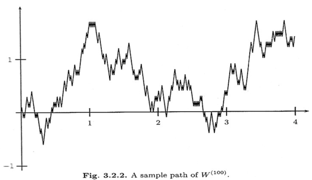
Figure 2: Scaled Symmetric Random Walk (source)

Since this is just a simple symmetric random walk (assuming we're analyzing it with its integer steps), the same properties hold as we discussed in Example 3. Namely, that non-overlapping increments are independent. Additionally, for \(0 \leq s \leq t\), we have:

\begin{align*} E[W^{(n)}(t) - W^{(n)}(s)] &= 0 \\ Var[W^{(n)}(t) - W^{(n)}(s)] &= t - s \\ \tag{2.14} \end{align*}

where we use the square root scaling to end up with variance accumulating still at one unit per time.

Another important property is called the quadratic variation, which is calculated along a specific path (i.e., there's no randomness involved). For a scaled symmetric random walk where we know the exact path it took up to time \(t\), we get:

\begin{align*} [W^{(n)}, W^{(n)}]_t &= \sum_{j=1}^{nt} (W^{(n)}(\frac{j}{n}) - W^{(n)}(\frac{j-1}{n}))^2 \\ &= \sum_{j=1}^{nt} [\frac{1}{\sqrt{n}} X_j]^2 \\ &= \sum_{j=1}^{nt} \frac{1}{n} = t \\ \tag{2.15} \end{align*}

This results in the same quantity as the variance computation we have (for \(s=0\)) in Equation 2.14 but is conceptually different. The variance is an average over all paths while the quadratic variation is taking a realized path, squaring all the values, and then summing them up. In the specific case of a Wiener process, they result in the same thing (not always the case for general stochastic processes).

Finally, as you might expect, we wish to understand what happens to the scaled symmetric random walk when \(n \to \infty\). For a given \(t\geq 0\), let's recall a few things:

• \(E[W^{(n)}(t)] = 0\) (from Equation 2.14 with \(s = 0\)).

• \(Var[W^{(n)}(t)] = t\) (from Equation 2.14 with \(s = 0\)).

• \(W^{(n)}(t) = \frac{1}{\sqrt{n}} \sum_{i=1}^t X_t\) for Bernoulli process \(X(t)\).

• The central limit theorem states that \(\frac{1}{\sqrt{n}}\sum_{i=1}^n Y_i\) converges to \(\mathcal{N}(\mu_Y, \sigma_Y^2)\) as \(n \to \infty\) for IID random variables \(Y_i\) (given some mild conditions).

We can see that our symmetric scaled random walk fits precisely the conditions as the central limit theorem, which means that as \(n \to \infty\), \(W^{(n)}(t)\) converges to a normal distribution with mean \(0\) and variance \(t\). This limit is in fact the method in which we'll define the Wiener process in the next subsection.

2.4.3 Quadratic Variation of Wiener Process

We looked at the quadratic variation above for the scaled symmetric random walk and concluded that it accumulates quadratic variation one unit per time (i.e., quadratic variation is \(T\) for \([0, T]\)) regardless of the value of \(n\). We'll see that this is also true for the Wiener process but before we do, let's first appreciate why this is strange.

Let \(f(t)\) be a function defined on \([0, T]\). The quadratic variation of \(f\) up to \(T\) is

\begin{equation*} [f, f](T) = \lim_{||\Pi|| \to 0} \sum_{j=0}^{n-1}[f(t_{j+1}) - f(t_j)]^2 \tag{2.18} \end{equation*}

for \(\Pi = \{t_0, t_1, \ldots, t_n\}\), \(0\leq t_1 \leq t_2 < \ldots < t_n = T\) and \(||\Pi|| = \max_{j=0,\ldots,n} (t_{j+1}-t_j)\).

This is basically the same idea that we discussed before: for infinitesimally small intervals, take the difference of the function for each interval, square them, and then sum them all up. Here we can have unevenly spaced partitions with the only condition being that the largest partition has to go to zero. This is called the mesh or norm of the partitions, which is similar to the formal definition of Riemannian integrals (even though many of us, like myself, didn't learn it this way). In any case, the idea is very similar to just having evenly spaced intervals that go to zero.

Now that we have Equation 2.18, let's see how it behaves on a function \(f(t)\) that has a continuous derivative: (recall the mean value theorem states that \(f'(c) = \frac{f(a) - f(b)}{b-a}\) for \(c \in (a,b)\) if \(f(x)\) is a continuous function with derivatives on the respective interval):

\begin{align*} [f, f](T) &= \lim_{||\Pi|| \to 0} \sum_{j=0}^{n-1}[f(t_{j+1}) - f(t_j)]^2 && \text{definition} \\ &= \lim_{||\Pi|| \to 0} \sum_{j=0}^{n-1}|f'(t_j^*)|^2 (t_{j+1} - t_j)^2 && \text{mean value theorem} \\ &\leq \lim_{||\Pi|| \to 0} ||\Pi|| \sum_{j=0}^{n-1}|f'(t_j^*)|^2 (t_{j+1} - t_j) \\ &= \big[\lim_{||\Pi|| \to 0} ||\Pi||\big] \big[\lim_{||\Pi|| \to 0} \sum_{j=0}^{n-1}|f'(t_j^*)|^2 (t_{j+1} - t_j)\big] && \text{limit product rule} \\ &= \big[\lim_{||\Pi|| \to 0} ||\Pi||\big] \int_0^T |f'(t)|^2 dt = 0&& f'(t) \text{ is continuous} \\ \tag{2.19} \end{align*}

So we can see that quadratic variation is not very important for most functions we are used to seeing i.e., ones with continuous derivatives. In cases where this is not true, we cannot use the mean value theorem to simplify quadratic variation and we potentially will get something that is non-zero.

For the Wiener process in particular, we do not have a continuous derivative and cannot use the mean value theorem as in Equation 2.19, so we end up with non-zero quadratic variation. To see this, let's take a look at the absolute value function \(f(t) = |t|\) in Figure 3. On the interval \((-2, 5)\), the slope between the two points is \(\frac{3}{7}\), but nowhere in this interval is the slope of the absolute value function \(\frac{3}{7}\) (it's either constant 1 or constant -1 or undefined).

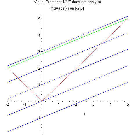
Figure 3: Mean value theorem does not apply on functions without derivatives (source)

Recall, this is a similar situation to what we had for the scaled symmetric random walk -- in between each of the discrete points, we used a linear interpolation. As we increase \(n\), this "pointy" behaviour persists and is inherited by the Wiener process where we no longer have a continuous derivative. Thus, we need to deal with this situation where we have a function that is continuous everywhere, but differentiable nowhere. This is one of the key reasons why we need stochastic calculus, otherwise we could just use the standard rules for calculus that we all know and love.

Theorem 1

For the Wiener process \(W\), the quadratic variation is \([W,W](T) = T\) for all \(T\geq 0\) almost surely.

Proof

Define the sampled quadratic variation for partition as above (Equation 2.18):

\begin{equation*} Q_{\Pi} = \sum_{j=0}^{n-1}\big( W(t_{j+1}) - W(t_j) \big)^2 \tag{2.20} \end{equation*}

This quantity is a random variable since it depends on the particular "outcome" path of the Wiener process (recall quadratic variation is with respect to a particular realized path).

To prove the theorem, we need to show that the sampled quadratic variation converges to \(T\) as \(||\Pi|| \to 0\). This can be accomplished by showing \(E[Q_{\Pi}] = T\) and \(Var[Q_{\Pi}] = 0\), which says that we will converge to \(T\) regardless of the path taken.

We know that each increment in the Wiener process is independent, thus their sums are the sums of the respective means and variances of each increment. So given that we have:

\begin{align*} E[(W(t_{j+1})-W(t_j))^2] &= E[(W(t_{j+1})-W(t_j))^2] - 0 \\ &= E[(W(t_{j+1})-W(t_j))^2] - E[W(t_{j+1})-W(t_j)]^2 && \text{definition of the Wiener process}\\ &= Var[W(t_{j+1})-W(t_j)] \\ &= t_{j+1} - t_j && \text{definition of the Wiener process}\\ \tag{2.21} \end{align*}

We can easily compute \(E[Q_{\Pi}]\) as desired:

\begin{align*} &E[Q_{\Pi}] \\ &= E[ \sum_{j=0}^{n-1}\big( W(t_{j+1}) - W(t_j) \big)^2 ] \\ &= \sum_{j=0}^{n-1} E[W(t_{j+1}) - W(t_j)]^2 \\ &= \sum_{j=0}^{n-1} (t_{j+1} - t_j) && \text{Equation } 2.21 \\ &= T \\ \tag{2.22} \end{align*}

From here, we use the fact that the expected value of the fourth moment of a normal random variable with zero mean is three times its variance. Anticipating the quantity we'll need to compute the variance, we have:

\begin{equation*} E\big[(W(t_{j+1})-W(t_j))^4 \big] = 3Var[(W(t_{j+1})-W(t_j)] = 3(t_{j+1} - t_j)^2 \tag{2.23} \end{equation*}

Computing the variance of the quadratic variation for each increment:

\begin{align*} &Var\big[(W(t_{j+1})-W(t_j))^2 \big] \\ &= E\big[\big( (W(t_{j+1})-W(t_j))^2 - E[(W(t_{j+1})-W(t_j))^2] \big)^2\big] && \text{definition of variance} \\ &= E\big[\big( (W(t_{j+1})-W(t_j))^2 - (t_{j+1} - t_j) \big)^2\big] && \text{Equation } 2.21 \\ &= E[(W(t_{j+1})-W(t_j))^4] - 2(t_{j+1}-t_j)E[(W(t_{j+1})-W(t_j))^2] + (t_{j+1} - t_j)^2 \\ &= 3(t_{j+1}-t_j)^2 - 2(t_{j+1}-t_j)^2 + (t_{j+1} - t_j)^2 && \text{Equation } 2.21/2.23 \\ &= 2(t_{j+1}-t_j)^2 \\ \tag{2.24} \end{align*}

From here, we can finally compute the variance:

\begin{align*} Var[Q_\Pi] &= \sum_{j=0}^{n-1} Var\big[ (W(t_{j+1} - W(t_j)))^2 \big] \\ &= \sum_{j=0}^{n-1} 2(t_{j+1}-t_j)^2 && \text{Equation } 2.24 \\ &\leq \sum_{j=0}^{n-1} 2 ||\Pi|| (t_{j+1}-t_j) \\ &= 2 ||\Pi|| T && \text{Equation } 2.22 \\ \tag{2.25} \end{align*}

As \(\lim_{||\Pi|| \to 0} Var[Q_\Pi] = 0\), therefore we have shown that \(\lim_{||\Pi|| \to 0} Q_\Pi = T\) as required.

The term almost surely is a technical term meaning with probability 1. This is another unintuitive idea when dealing with infinities. The theorem doesn't say that there are no paths with different quadratic variation, it only says those paths are negligible in size with respect to the infinite number of paths, and thus have probability zero.

Taking a step back, this is quite a profound result: if you take any realized path of the Wiener process, sum the infinitesimally small squared increments of that paths, it equals the length of the interval almost surely. In other words, the Wiener process accumulates quadratic variation at a rate of one unit per time.

This is perhaps surprising result because it can be any path. It doesn't matter how the "infinitely fast" coin flips land, the sum of the square increments will always approach the length of the interval. The fact that it's also non-zero is surprising too despite the path being continuous (but without a continuous derivative) as we discussed above.

We often will informally write:

\begin{equation*} dW(t)dW(t) = dt \tag{2.26} \end{equation*}

To describe the accumulation of quadratic variation at one unit per time. However, this should not be interpreted to be true for each infinitesimally small increment. Recall each increment of \(W(t)\) is normally distributed, so the LHS of Equation 2.26 is actually distributed as the square of a normal distribution. We only get the result of Theorem 1 when we sum a large number of them (see [1] for more details).

We can also use this informal notation to describe a few other related concepts. The cross variation (Equation 2.27) and quadratic of variation for the time variable (Equation 2.28) respectively:

\begin{align*} dW(t)dt &= 0 \tag{2.27} \\ dtdt &= 0 \tag{2.28} \end{align*}

The quadratic variation for time can use the same definition from Equation 2.18 above, and the cross variation just uses two different function (\(W(t)\) and \(t\)) instead of the same function. Intuitively, both of these are zero because the time increment (\(\Pi\)) goes to zero in the limit by definition, thus so do these two variations. This can be shown more formally using similar arguments as the quadratic variation above (see [1] for more details).

2.5 The Relationship Between the Wiener Process and White Noise

The Wiener process can be characterized in several equivalent ways with the definition above being one of the most common. Another common way to define it is from the white noise we discussed in the motivation section. In this definition, the Wiener process is the definite integral of Gaussian white noise, or equivalently, Gaussian white noise is the derivative of the Wiener process:

To understand why this relationship is true, let's first define the derivative of a stochastic process from [4]:

A stochastic process \(X(t)\), \(t \in \mathbb{R}\), is said to be differentiable in quadratic mean with derivative \(X'(t)\) if

\begin{align*} \frac{X(t+h) - X(t)}{h} &\to X'(t) \\ E\big[(\frac{X(t+h) - X(t)}{h} - X'(t))^2 \big] &\to 0 \\ \tag{2.31} \end{align*}

when \(h \to 0\).

We can see that the definition is basically the same as regular calculus except that we require the expectation to go to zero with a weaker squared convergence, which we'll see appear again in the next section.

From this definition, we can calculate the mean of the derivative of \(W(t)\) as:

Similarly, we can show a general property about the time correlation of a derivative of a stochastic process:

Thus we have shown that the time correlation of the derivative of a stochastic process is the mixed second-order partial derivative. Now all we have to do is evaluate it for the Wiener process.

First, assuming \(t_1 < t_2\) the Wiener process time correlation is given by (see this StackExchange answer for more details):

We get the same result if \(t_2 < t_1\), thus \(C_W(t_1, t_2) = \min(t_1, t_2)\). Now we have to figure out how to take the second order partial derivatives. The first partial derivative is easy as long as \(t_1 \neq t_2\) (see this answer on StackExchange):

where \(H(x)\) is the Heaviside step function. But we know the derivative of this step function is just the Dirac delta function (even with the missing point), so:

From Equation 2.32 and 2.36, we see we have the same statistics as the white noise we defined in the motivation section above in Equation 1.4. Since the mean is also zero, the covariance is equal to the time correlation too: \(Cov_{W'}(t_1, t_2) = C_{W'}(t_1, t_2)\)

Now all we have to show is that it is also normally distributed. By definition (given above) the Wiener stochastic process has derivative:

But since each increment of the Wiener process is normally distributed (and independent), the derivative from Equation 2.37 is also normally distributed since the difference of two independent normals is normally distributed. This implies the derivative of the Wiener process is a Gaussian process with zero mean and delta time correlation, which is the standard definition of Gaussian white noise. Thus, we have shown the relationship in Equation 2.29 / 2.30.

2.6 The Importance of the Wiener Process

One question that you might ask (especially after reading the next section) is why is there so much focus on the Wiener process? It turns out that the Wiener process is the only (up to a scaling factor and drift term) continuous process with stationary independent increments [5]. Let's be more precise.

A stochastic process is said to have independent increments if \(X(t) - X(s)\) is independent of \(\{X(u)\}_{u\leq s}\) for all \(s\leq t\). If the distribution of the increments don't depend on \(s\) or \(t\) directly (but can depend on \(t-s\)), then the increments are called stationary. This leads us to this important result:

Equation 2.38 is the generalized Wiener process that includes a potentially non-zero initial value \(X(0)\), deterministic drift term \(bt\), and scaling factor \(\sigma\).

The intuition behind Theorem 3 follows directly from the central limit theorem. For a given interval \([s, t]\), the value of \(X(t) - X(s)\) is the sum of infinitesimally small independent, identically distributed partitions, or in other words IID random variables (doesn't have to be normally distributed). Thus, we can apply the central limit theorem and get a normal distribution (under some mild conditions).

Processes with independent increments appear in many contexts. For example, the random displacement of a macro particle moving through a fluid caused by the random interactions with the fluid molecules is naturally modelled using the Wiener process. Similarly, the variability of the return of a stock price in a very short period of time is approximately the same regardless of the price, thus can also be modelled using a Wiener process. We'll look at both of these examples more closely later on in the post.

3.1 Stochastic Integrals with Brownian Motion

To begin, we'll start with the simplest case when the integrator (\(dX(t)\) in Equation 3.1) is the Wiener process. For this simple case, we can define the integral as:

where \(t_j \leq s_j \leq t_{j+1}\), and \(||\Pi||\) is the mesh (or maximum partition) that goes to zero while the number of partitions goes to infinity like in Equation 2.18 (and standard Riemannian integrals).

From a high level, Equation 3.2 is not too different from our usual Riemannian integrals. However, we have to note that instead of having a \(dt\), we have a \(dW(s)\). This makes the results more volatile than a regular integral. Let's contrast the difference between approximating a regular and stochastic integral for a small step size \(\Delta t\) starting from \(t\):

\(R(t)\) changes more predictably than \(I(t)\) since we know that each increment changes by \(H(s)\Delta t\). Note that \(H(s)\) can still be a random (and \(R(t)\) can be random as well) but its change is multiplied by a deterministic \(\Delta t\). This is in contrast to \(I(t)\) which changes by \(W(t + \Delta t) - W(t)\). Recall that each increment of the Wiener process is independent and distributed normally with \(\mathcal{N}(0, \Delta t)\). Thus \(H(t)(W(t + \Delta t) - W(t))\) changes much more randomly and erratically because our increments follow an independent normal distribution versus just a \(\Delta t\). This is one of the key intuitions why we need to define a new type of calculus.

To ensure that the stochastic integral in Equation 3.2 is well defined, we need a few conditions, which I will just quickly summarize:

1. The choice of \(s_j\) is quite important (unlike regular integrals). The Itô integral uses \(s_j = t_j\), which is more common in finance; the Stratonovich integral uses \(s_j = \frac{(t_j + t_{j+1})}{2}\), which is more common in physics. We'll be using the Itô integral for most of this post, but will show the difference in the example below.

2. \(H(t)\) must be adapted to the same process as our integrator \(X(t)\), otherwise we would be allowing it to "see into the future". For most of our applications, this is a very reasonable assumption.

3. The integrand needs to have square-integrability: \(E[\int_0^T H^2(t)dt] < \infty\).

4. We ideally want to ensure that each sample point of the integrand \(H(s_j)\) from Equation 3.2 converges in the limit to \(H(s)\) with probability one (remember we're still working with stochastic processes here). That's a pretty strong condition, so we'll actually use a weaker squared convergence as:

   \begin{equation*} \lim_{n \to \infty} E\big[\int_0^T |H_n(t) - H(t)|^2 dt\big] = 0 \tag{3.5} \end{equation*}

   where we define \(H_n(s) := H(t_j)\) for \(t_j \leq s < t_{j+1}\) i.e., it's the constant piece-wise approximation for \(H(t)\) using the left most point for the interval.

3.2 Itô Processes and Integrals

In the previous subsections, we only allowed integrators that were Wiener processes but we'd like to extend that to a more general class of stochastic processes called Itô processes 2:

Let \(W(t)\), \(t\geq 0\), be a Wiener process with an associated filtration \(\mathcal{F}(t)\). An Itô process is a stochastic process of the form:

\begin{equation*} X(t) = X(0) + \int_0^t \mu(s) ds + \int_0^t \sigma(s) dW(s) \tag{3.16} \end{equation*}

where \(X(0)\) is nonrandom and \(\sigma(s)\) and \(\mu(s)\) are adapted stochastic processes.

Equation 3.16 can also be written in its more natural (informal) differential form:

A large class of stochastic processes are Itô processes. In fact, any stochastic process that is square integrable measurable with respect to a filtration generated by a Wiener process can be represented by Equation 3.16 (see the martingale representation theorem). Thus, many different types of stochastic processes that we practically care about are Itô processes.

Using our differential notation, we can take Equation 3.17 and take the expectation and variance to get more insight:

In Equation 3.18, \(\sigma(t)\) and \(dW(t)\) are independent because \(\sigma(t)\) is adapted to \(W(t)\), thus the \(dW(t)\) increment is in the "future" of the current value of \(\sigma(t)\). This reasoning only works because of the choice of the \(s_j=t_j\) in Equation 3.2 for the Itô integral.

In fact, this result actually holds if we convert to our integral notation:

So the notation of using \(\mu\) and \(\sigma\) makes more sense. The regular time integral contributes to the mean of the Itô process, while the stochastic integral contributes to the variance. We'll see how we can practically manipulate them in the next section.

Lastly as with our other processes, we would like to know its quadratic variation. Informally we can compute quadratic variation as:

which is essentially the same computation we used in Equation 3.19 above (and the same as the variance). In fact, we get the same result as with the simpler Wiener process where we accumulate quadratic variation with \(H^2(t)\) per unit time. The reason is that the cross variation (Equation 2.27) and time quadratic variation (Equation 2.28) are zero and don't contribute to the final expression.

Finally, let's see how to compute an integral of an Itô process \(X(t)\) using our informal differential notation:

As we can see, it's just a sum of a simple Wiener process stochastic integral and a regular time integral.

3.3 Itô's Lemma

Although many stochastic processes can be written as Itô processes, often times the process under consideration is not in the form of Equation 3.16/3.17. A common situation is where our target stochastic process \(Y(t)\) is a deterministic function \(f(\cdot)\) of a simpler Itô process \(X(t)\):

In these situations, we'll want a method to simplify this so we can get it into the simpler form of Equation 3.16/3.17 with a single \(dt\) and a single \(dW(s)\) term. This technique is known as Itô's lemma.

As you can see, we can re-write the above stochastic process from Equation 3.28 in terms of a single \(dt\) and single \(dW(s)\) term (using differential notation). This can be thought of as a form of the chain rule for total derivatives, except now that we have a non-zero quadratic variation, we need to include the extra second order term involving \(dW(s)dW(s)\).

Itô's lemma is an incredibly important result because most applications of stochastic calculus are "little more than repeated use of this formula in a variety of situations" [1]. In fact, based on what I can tell, many introductory courses to stochastic calculus skip over a lot of the theoretical material and simply just jump directly into applications of Itô's lemma because that's mostly what you need.

3.4 Stochastic Differential Equations

One of the most common problems we want to use stochastic calculus for is solving stochastic differential equations (SDE). Similar to their non-stochastic counterpart, they appear in many different phenomenon (a couple of which we will see in the next section) and are usually very natural to write, but not necessarily to easy solve.

Starting with the definition:

A stochastic differential equation is an equation of the form:

\begin{align*} dX(t) &= \mu(t, X(t))dt + \sigma(t, X(t)) dW(t) && \text{differential form}\tag{3.35} \\ X(T) &= X(t) + \int_t^T \mu(u, X(u))du + \int_t^T \sigma(u, X(u)) dW(u) && \text{integral form} \tag{3.36} \end{align*}

where \(\mu(t, x)\) and \(\sigma(t, x)\) are given functions called the drift and diffusion respectively. Additionally, we are given an initial condition \(X(t) = x\) for \(t\geq 0\). The problem is to then find the stochastic process \(X(T)\) for \(T\geq t\).

Notice that \(X(t)\) appears on both sides making it difficult to solve for explicitly. A nice property though is that under mild conditions on \(\mu(t, x)\) and \(\sigma(t, x)\), there exists a unique process \(X(T)\) that satisfies the above. As you might also guess, one-dimensional, linear SDEs can be solved for explicitly.

SDEs can add similar complexities as their non-stochastic counterparts such as non-linearities, systems of SDEs, and multidimensional SDEs (with multiple associated Wiener processes) etc. Generally, SDEs won't have explicit closed form solutions so you'll have to use numerical methods to solve them.

The two popular methods are Monte Carlo simulation and numerically solving a partial differential equation (PDE). Roughly, Monte Carlo simulation for differential equations involve simulating many different paths of the underlying process and using these paths to compute the associated statistics (e.g., mean, variance etc.). Given enough paths (and associated time), you generally can get as accurate as you like.

The other method is to numerically solve a PDE. An SDE can be recast to as a PDE problem (at least in finance applications, not sure about others), and from the PDEs you can use the plethora of numerical methods to solve them. How both of these methods work is beyond the scope of this post (and how far I wanted to dig into this subject), but there is a lot of literature online about it.

4.1 Black-Scholes-Merton Model for Options Pricing

The rigorous math to get to the Black-Scholes-Merton model for options pricing is quite in depth so instead I'll just present a quick overview of some of the main concepts and intuition (following [6] closely). See [6] for a lighter but more intuitive treatment, and [1] for all the gory details.

4.2 Langevin Equation

A Langevin equation is a well known stochastic differential equation that describes how a system evolves when subjected to a combination of deterministic and fluctuating forces. The original equation was developed well before stochastic calculus was discovered in the context of the apparent random movement of a particle through a fluid, which describes the physical phenomenon of Brownian motion. Since the Wiener process and Brownian motion are so related, they are sometimes used interchangeably to describe the underlying stochastic process.

Many people contributed to the discovery of Brownian motion (including Einstein) but the stochastic differential equation was derived several years after by Langevin (hence the name) in 1908. Interestingly, since Langevin did not approach his stochastic differential equation with much rigour (by mathematician standards), this gave rise to the field of stochastic analysis to answer some of the issues with Langevin's approach.

In this section, I'm going to give a brief overview of the Langevin equation in the context of Brownian motion, glossing over many of the usual analyses one would do in a physics class. Additionally, I'm going to approach it using Itô calculus, which is not the typical approach (not the one originally used). Finally, I'll briefly mention its relationship to a financial application.