Variational Autoencoders

This post is going to talk about an incredibly interesting unsupervised learning method in machine learning called variational autoencoders. It's main claim to fame is in building generative models of complex distributions like handwritten digits, faces, and image segments among others. The really cool thing about this topic is that it has firm roots in probability but uses a function approximator (i.e. neural networks) to approximate an otherwise intractable problem. As usual, I'll try to start with some background and motivation, include a healthy does of math, and along the way try to convey some of the intuition of why it works. I've also annotated a basic example so you can see how the math relates to an actual implementation. I based much of this post on Carl Doersch's tutorial, which has a great explanation on this whole topic, so make sure you check that out too.

1. Generative Models

The first thing to discuss is the idea of a generative model. A generative model is a model which allows you to sample (i.e. randomly generate data points) from a distribution similar to your observed (i.e. training) data. We can accomplish this by specifying a joint distribution over all the dimensions of the data (including the "y" labels). This allows us to generate any number of data points that has similar characteristics to our observed data. This is in contrast to a discriminative model, which can only model dependence between the outcome variable (\(y\)) and features (\(X\)). For example, a binary classifier only outputs 0 or 1 "y" labels and cannot generate a data point that looks like your "X" features.

Typically, as part of your model you'll want to specify latent variables that represent some higher level concepts. This allows for intuitive relationships between the latent variables and the observed ones, while usually simplifying the overall number of parameters (i.e. complexity) of the model. We'll be focusing on the application of generating new values that look like the observed data but check out the Wikipedia article for a better picture of some other applications.

2. An Implicit Generative Model (aka the "decoder")

Let's continue to use this handwritten digit as our motivation for generative models. Generating a 28x28 greyscale image that looks like a digit is non-trivial, especially if we are trying to model it directly. The joint distribution over 28x28 random variables is going to be complex, for example, enforcing that "0"s have empty space near the middle but "1"s don't, is not an easy thing to do. Typically in these situations, we'll introduce latent variables which encode higher level ideas. In our example, one of the latent variables might correspond to which digit we're using (0-9), another one may be the stroke width we use, etc. This model is simpler because there are usually fewer parameters to estimate, reducing the number of data points required for a good fit. (See my post on the expectation-maximization algorithm, which has a brief description of latent variable models in the background section)

One of the downsides of any latent variable model is that you have to specify the model! That is, you have to have some idea of what latent variables you want to include, how these variables are related to each other and the observed variables, and finally how to fit the model (which depends on the connectivity). All of these issues introduce potential for a misspecification of the model. For example, maybe you forgot to include stroke width and now all your handwritten digits are blurry because it averaged over all the types of stroke widths in your training dataset. Wouldn't it be nice if you didn't need to explicitly specify the latent variables (and associated distributions), nor the relationships between them, and on top of all of this had an easy way to fit the model? Enter variational autoencoders.

2.1 From a Standard Normal Distributions to a Complex Latent Variable Model

There are a couple of big ideas here that allow us to create this implicit model without explicitly specifying anything. The first big idea here is that we're not going to explicitly define any latent variables, that is, we won't say "this variable is for digit 0", "this one for digit 1", ..., "this variable is for stroke width", etc. Instead, we'll have our latent variables as a simple uninterpretable standard isotropic multivariate normal distribution \(\mathcal{N}(0, I)\) where \(I\) is the identify matrix. You may be wondering how we can ever model anything complex if we just use a normal distribution? This leads us to the next big idea.

The second big idea is that starting from any random variable \(Z\), there exists a deterministic function \(Y=g(Z)\) (under most conditions) such that \(Y\) can be any complex target distribution you want (see the box on "Inverse Transform Sampling" below). The ingenious idea here is that we can learn \(g(\cdot)\) from the data! Thus, our variational autoencoder can transform our boring, old normal distribution into any funky shaped distribution we want! As you may have already guessed, we use a neural network as a function approximator to learn \(g(\cdot)\).

The last little bit in defining our latent variable model is translating our latent variable into the final distribution of our observed data. Here, we'll also use something simple: we'll assume that the observed data follows a isotropic normal distribution \(\mathcal{N}(g(z), \sigma^2 * I)\), with mean following our learned latent random variable from the output of \(g\), and identity covariance matrix scaled by a hyperparameter \(\sigma^2\).

The reason why we want to put a distribution on the output is that we want to say that our output is like our observed data -- not exactly equal. Remember, we're using a probabilistic interpretation here, so we need to write a likelihood function and then maximize it, usually by taking its gradient. If we didn't have an output distribution, we would implicitly be saying that \(g(z)\) was exactly equal i.e. a Dirac delta function, which would result in a discontinuity. This is important because we will eventually want to use stochastic gradient descent to learn \(g(z)\) and this implicitly requires a smooth function. We'll see how this probabilistic interpretation plays into the loss/objective function below.

Inverse Transform Sampling

Inverse transform sampling is a method for sampling from any distribution given its cumulative distribution function (CDF), \(F(x)\). For a given distribution with CDF \(F(x)\), it works as such:

1. Sample a value, \(u\), between \([0,1]\) from a uniform distribution.

2. Define the inverse of the CDF as \(F^{-1}(u)\) (the domain is a probability value between \([0,1]\)).

3. \(F^{-1}(u)\) is a sample from your target distribution.

Of course, this method has no claims on being efficient. For example, on continuous distributions, we would need to be able to find the inverse of the CDF (or some close approximation), which is not at all trivial. Typically, there are more efficient ways to perform sampling on any particular distribution but this provides a theoretical way to sample from any distribution.

Proof

The proof of correctness is actually pretty simple. Let \(U\) be a uniform random variable on \([0,1]\), and \(F^{-1}\) as before, then we have:

\begin{align*} &P(F^{-1}(U) \leq x) \\ &= P(U \leq F(x)) && \text{apply } F \text{ to both sides} \\ &= F(x) && \text{because } P(U\leq y) = y \text{ on } [0,1] \\ \tag{3} \end{align*}

Thus, we have shown that \(F^{-1}(U)\) has the distribution of our target random variable (since the CDF \(F(x)\) is the same).

It's important to note what we did: we took an easy to sample random variable \(U\), performed a deterministic transformation \(F^{-1}(U)\) and ended up with a random variable that was distributed according to our target distribution.

Example

As a simple example, we can try to generate a exponential distribution with CDF of \(F(x) = 1 - e^{-\lambda x}\) for \(x \geq 0\). The inverse is defined by \(x = F^{-1}(u) = -\frac{1}{\lambda}\log(1-y)\). Thus, we can sample from an exponential distribution just by iteratively evaluating this expression with a uniform randomly distributed number.

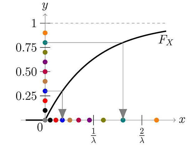
Figure 1: The \(y\) axis is our uniform random distribution and the \(x\) axis is our exponentially distributed number. You can see for each point on the \(y\) axis, we can map it to a point on the \(x\) axis. Even though \(y\) is distributed uniformly, their mapping is concentrated on values closer to \(0\) on the \(x\) axis, matching an exponential distribution (source: Wikipedia).

Extensions

Now instead of starting from a uniform distribution, what happens if we want to sample from another distribution, say a normal distribution? We just first apply the reverse of the inverse sampling transform called the Probability Integral Transform. So the steps would be:

1. Sample from a normal distribution.

2. Apply the probability integral transform using the CDF of a normal distribution to get a uniformly distributed sample.

3. Apply inverse transform sampling with the inverse CDF of the target distribution to get a sample from our target distribution.

What about extending to multiple dimensions? We can just break up the joint distribution into its conditional components and sample each sequentially to construct the overall sample:

\begin{equation*} P(x_1,\ldots, x_n) = P(x_n|x_{n-1}, \ldots,x_1)\ldots P(x_2|x_1)P(x_1) \tag{4} \end{equation*}

In detail, first sample \(x_1\) using the method above, then \(x_2|x_1\), then \(x_3|x_2,x_1\), and so on. Of course, this implicitly means you would have the CDF of each of those distributions available, which practically might not be possible.

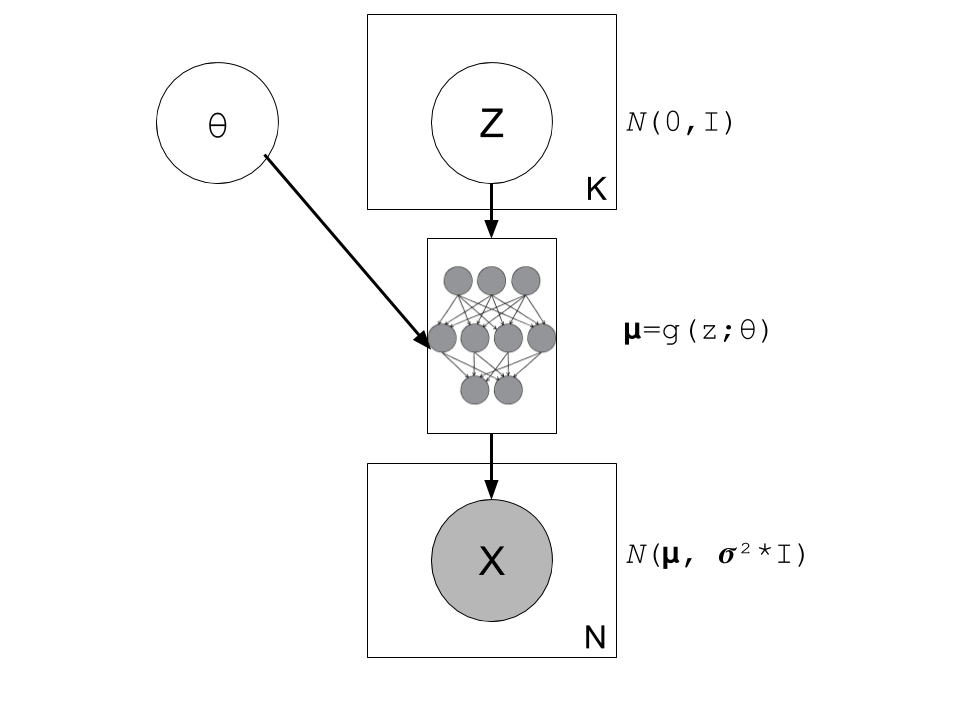
Figure 2: A graphical model of a typical variational autoencoder (without a "encoder", just the "decoder"). We're using a modified plate notation: the circles represent variables/parameters, rectangular boxes with a number in the lower right corner to represent multiple instances of the contained variables, and the little diagram in the middle is a representation of a deterministic neural network (function approximator).

Writing the model out more formally, we have:

where:

• \(X_{i=1,\ldots,N}\) are our normally distributed observations

• \(\mu_{i=1,\ldots,N}\) are the mean of our observed variables which potentially has a very complex distribution

• \(\sigma^2\) is a hyperparameter

• \(I\) is the identify matrix

• \(g(Z_{1,\ldots,K}; \theta)\) is a deterministic function with parameters to be learned \(\theta\) (e.g. weights of a neural network)

• \(Z_{i=1,\ldots,K}\) are standard isotropic normally distributed random variables

Note: we can put another distribution on \(X\) like a Bernoulli for binary data parameterized by \(p=g(z;\theta)\). The important part is we're able to maximize the likelihood over the \(\theta\) parameters. Implicitly, we will want our output variable to be continuous in \(\theta\) so we can take its gradient.

2.2 A hard fit

Given the model above, we have all we need to fit the model: observations from \(X\), fully defined latent variables (\(Z\)), and a function approximator \(g(\cdot)\); the only thing we need to find is \(\theta\). This is a classic optimization problem where we could use an MLE (or MAP) estimate. Let's see how this works out.

First, we need to define the probability of seeing a single example \(x\):

The probability of a single sample is just the joint probability of our given model marginalizing (i.e. integrating) out \(Z\). Since we don't have an analytical form of the density, we approximate the integral by averaging over \(M\) samples from \(Z\sim \mathcal{N}(0, I)\).

Putting together the log-likelihood (defined by log'ing the density and summing over all of our \(N\) observations):

Two problems here. First, the \(\log\) can't be pushed inside the summation, which actually isn't much a problem because we're not trying to derive an analytical expression here; so long as we can use gradient descent to learn \(\theta\), we're good. In this case, we can easily take derivatives since our density is normally distributed.

The other big problem, that is not easily seen through the notation, is that \(z_m\) is actually a \(K\)-dimensional vector. In order to approximate the integral properly, we would have to sample over a huge number of \(z\) values for each \(x_i\) sample! This basically plays into the curse of dimensionality whereby each additional dimension of \(z\) exponentially increases the number of samples you need to properly approximate the volume of the space. For small \(K\) this might be feasible but any reasonable value, it will be intractable.

Looking at it from another point of view, the reason why this is intractable is because it's inefficient; for each \(x\), we have to average over a large number (\(M\)) samples. But, for any given observation \(x\), most of the \(z_m\) will contribute very little to the likelihood. Using the handwritten digit example, if we're trying to generate a "0", most of the values of \(z_m\) sampled from our prior will have a very small probability of generating a "0", so we're wasting a lot of computation in trying to average over all these samples 1.

Wouldn't it be nice if we could just sample from \(p(z|X=x_i)\) directly and only pick \(z\) values that contribute a significant amount to the likelihood, thus getting rid the need for the large inefficient summation over \(M\) samples? This is exactly what variational autoencoders proposes!

(Note: Just to be clear, each \(x_i\) will likely have a different \(p(z|X=x_i)\). Imagine our hand written digit example, a "1" will probably have a very different posterior shape than an "8".)

2.2 Summary

To summarize, this is what we're trying to accomplish:

• Our generative model is an implicit latent variable model with latent variables \(Z\) as standard isotropic multivariate normal distribution.

• The \(Z\) variables are transformed into an arbitrarily complex distribution by a deterministic function approximator (e.g. neural network parameterized by \(\theta\)) that can model our data.

• We can fit our generative model via the likelihood by averaging over a huge number of \(Z\) samples; this becomes intractable for higher dimensions (curse of dimensionality).

• For any given sample \(x_i\), most of the \(z\) samples will contribute very little to the likelihood calculation, so we wish to sample only the probable values of \(z_m\) that contribute significantly to the likelihood using the posterior distribution \(z|X=x_i\).

From here, we can finally get to the "variational" part of variational autoencoders.

3. Variational Bayes for the Posterior (aka the "encoder")

From our novel idea of an implicit generative model, we come to a new problem: how can we estimate the posterior distribution \(Z|X=x_i\)? We have a couple of problems, first, the posterior probably has no closed form analytic solution. This is not terrible because this is a typical problem in Bayesian inference which we solve via either Markov Chain Monte Carlo Methods or Variational Bayes. Second, we wanted to use the posterior \(Z|X=x_i\) to maximize our likelihood function \(P(X|Z;\theta)\), but surely to find \(Z|X=x_i\) we need to know \(X|Z\) -- a circular dependence. The solution to this is also novel, let's simultaneously, fit our posterior, generate samples from it, and maximize our original log-likelihood function!

First, we'll attempt to solve the first problem of finding the posterior \(P(z|X=x_i)\) and this will lead us to the solution to the second problem of fitting our likelihood. Let's dig into some math to see how this works.

3.1 Setting up the Variational Objective

Since the posterior is so complex, we won't try to model it exactly. Instead, we'll use variational Bayesian methods (see my previous post) to approximate it. We'll denote our approximate distribution as \(Q(Z|X)\) and, as usual, we'll use KL divergence as our measure of "closeness" to the actual distribution. Writing the math down, we get:

We pulled \(P(X)\) out of the expectation since it is not dependent on \(z\). Rearranging Equation 8:

where we use the definition of KL divergence on the RHS. This is the core objective of variational autoencoders for which we wish to maximize. The LHS defines our higher level goal:

• \(\log P(X)\): maximize the log-likelihood (Equation 7)

• \(\mathcal{D}(Q(z|X) || P(z|X))\): Minimize the KL divergence between our approximate posterior \(Q(z|X)\) to fit \(P(z|X)\)

The RHS gives us an explicit objective where we know all the pieces, and we can maximize via gradient descent (details in the next section):

• \(P(X|z)\): original implicit generative model

• \(Q(z|X)\): approximate posterior (we'll define what this looks like below)

• \(P(z)\): prior distribution of latent variables (standard isotropic normal distribution)

Notice, we now have what appears to be an "autoencoder". \(Q(z|X)\) "encodes" \(X\) to latent representation \(z\), and \(P(X|z)\) "decodes" \(z\) to reconstruct \(X\). We'll see how these equations translate into a model that we can directly optimize.

3.2 Defining the Variational Autoencoder Model

Now that we have a theoretical framework that gives us an objective to optimize, we need to explicitly define \(Q(z|X)\). In the same way we implicitly defined the generative model, we'll use the same idea to define the approximate posterior. We'll assume that the Q(z|X) is normally distributed with mean and co-variance matrix defined by a neural network with parameters \(\phi\). The co-variance matrix is usually constrained to be diagonal to simplify things a bit. Formally, we'll have:

where:

• \(z|X\) is our approximated posterior distribution as a multivariate normal distribution

• \(\mu_{z|X}\) is a vector of means for our normal distribution

• \(\Sigma_{z|X}\) is a diagonal co-variance matrix for our normal distribution

• \(g_{z|X}\) is our function approximator (neural network)

• \(\phi\) are the parameters to \(g_{z|X}\)

As a first attempt, we might try to put Equations 5 and 10 to form a model as shown in Figure 3. The red boxes show our variational loss (objective) function from Equation 9 (Note: the squared error comes from the \(\log\) of the normal distribution and KL divergence between two multivariate normals is well known); the input and the sampling of the \(z\) values is shown in blue.

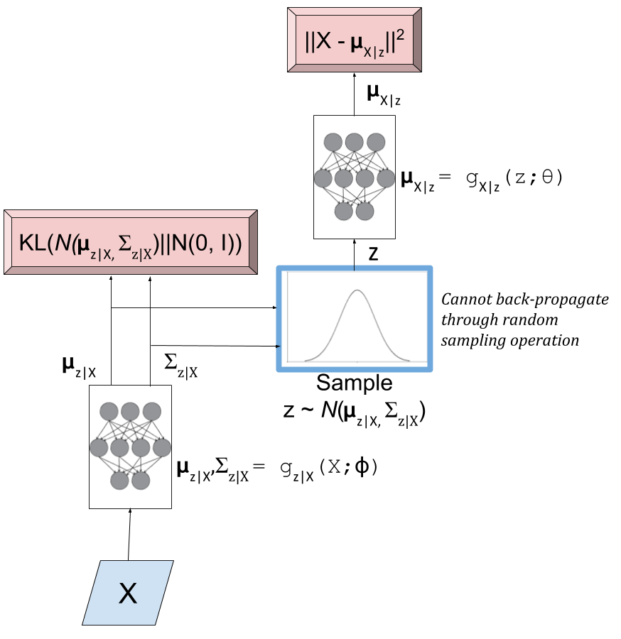
Figure 3: An initial attempt at a variational autoencoder without the "reparameterization trick". Objective functions shown in red. We cannot back-propagate through the stochastic sampling operation because it is not a continuous deterministic function.

Using this model, we can perform a "forward pass":

1. Inputting values of \(X=x_i\)

2. Computing \(\mu_{z|X}\) and \(\Sigma_{z|X}\) from \(g_{z|X}(X;\phi)\)

3. Sample a \(z\) value from \(\mathcal{N}(\mu_{z|X}, \Sigma_{z|X})\)

4. Compute \(\mu_{X|z}\) from \(g_{X|z}(z;\theta)\) to produce the (mean of the) reconstructed output.

Remember, our goal is to learn the parameters for our two networks: \(\theta\) and \(\phi\). We can attempt to do this through back-propagation but we hit a road-block when we back-propagate the \(||X-\mu_{X|z}||^2\) error through the sampling operation. Since the sampling operation isn't a continuous deterministic function, it has no gradient, thus we can't do any form of back-propagation. Fortunately, we can use the "reparameterization trick" to circumvent this sampling problem. This is shown in Figure 4.

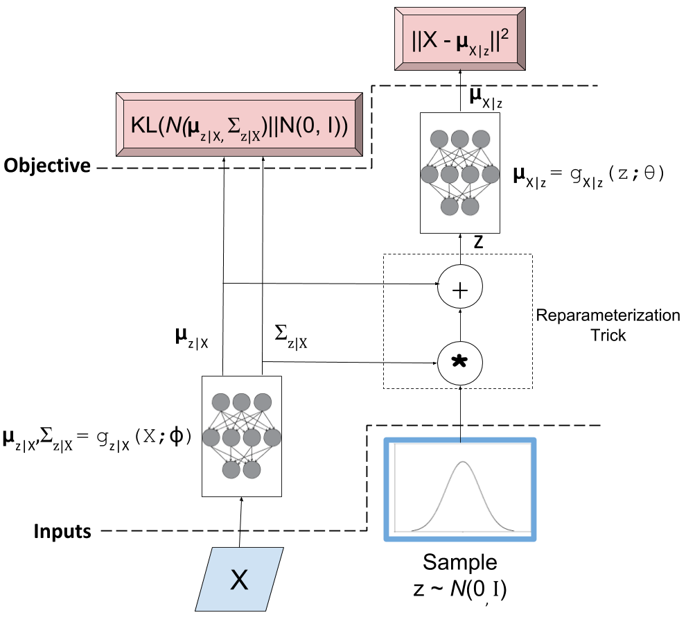
Figure 4: A variational autoencoder with the "reparameterization trick". Notice that all operations between the inputs and objectives are continuous deterministic functions, allowing back-propagation to occur.

The key insight is that \(\mathcal{N}(\mu_{z|X}, \Sigma_{z|X})\) is equivalent to \(\mathcal{N}(0, I) * \Sigma_{z|X} + \mu_{z|X}\). That is, we can just sample from an standard isotropic normal distribution and then scale and shift our sample to transform it to a sample from our desired \(z|X\) distribution. Shifting the sampling operation to an input of our model (for each sample \(x_i\), we can sample an arbitrary number of \(\mathcal{N}(0,I)\) samples to pair with it).

With the "reparameterization trick", this new model allows us to take the gradient of the loss function with respect to the target parameters (\(\theta\) and \(\phi\)). In particular, we would want to take these gradients:

and iteratively update the weights of our neural network using back-propagation. As seen in Figure 4, \(Q(z|X) = N(\mu_{z|X}, \Sigma_{z|X})\) is parameterized by \(\phi\) via \(g_{z|X}(X;\phi)\), whereas \(\mu_{X|z}\) is implicitly parameterized by both \(\theta\) through via \(g_{X|z}(z;\theta)\), and \(\phi\) through \(z\) and \(g_{z|X}(X;\phi)\).

3.3 Training a Variational Autoencoder

Now that we have the basic structure of our network and understand the relationship between the "encoder" and "decoder", let's figure out how to train this sucker. Recall Equation 9 shows us how define our objective in terms of distributions: \(z, z|X, X|z\). When we're optimizing, we don't directly work with distributions, instead we have samples and a single objective function. We can translate Equation 9 into this goal by taking the expectation over the relevant variables like so:

To be a bit pedantic, we still don't have a function we can't optimize directly because we don't know how to take the expectation. Of course, we'll just make the usual approximations by replacing the expectation with summations. I'll show it step by step, starting from the RHS of Equation 12:

Going line by line: first, we use our "reparameterization trick" by just sampling from our isotropic normal distribution instead of our prior \(z\). Next, let's approximate the outer expectation by taking our N observations of the \(X\) values and averaging them. This is what we implicitly do in most learning algorithms when we assume i.i.d. Finally, we'll simplify the inner expectation by just using a single sample paired with each observation \(x_i\). This requires a bit more explanation.

We want to simplify the inner expectation \(E_{\epsilon \sim \mathcal{N}(0, I)}[\cdot]\). To compute this, each time we evaluate the network, we must explicitly sample a new value of \(\epsilon\) from our isotropic normal distribution. That means we can just pair each observation \(x_i\) with a bunch of samples from \(\mathcal{N}(0, I)\) to make a "full input".

However, instead of doing that explicitly, let's just pair each \(x_i\) with a single sample from \(\mathcal{N}(0, I)\). If we're training over many epochs (large loop over all \(x_i\) values), it's as if we are pairing each observation with a bunch of new values sampled from \(\mathcal{N}(0, I)\). According to stochastic gradient descent theory, these two methods should converge to the same place and it simplifies life for us a bit.

As a final note, we can simplify the last line in Equation 13 to something like:

Each of the two big terms corresponds to \(\log P(x_i|z)\) and \(\mathcal{D}(Q(z|x_i) || P(z)\) respectively, where I dropped out some of the constants from \(\log P(x_i|z)\) (since they're not needed in the gradient) and used the formula for KL divergence between two multivariate normals.

And now that we have a concrete formula for the overall objective, it's straight forward to perform stochastic gradient descent either by manually working the derivatives or using some form of automatic differentiation.

3.4 Generating New Samples

Finally, we get to the interesting part of our model. After all that training we can finally try to generate some new observations using our implicit generative model. Even though we did all that work with the "reparameterization trick" and KL divergence, we still only need our implicit generative model from Section 2.1.

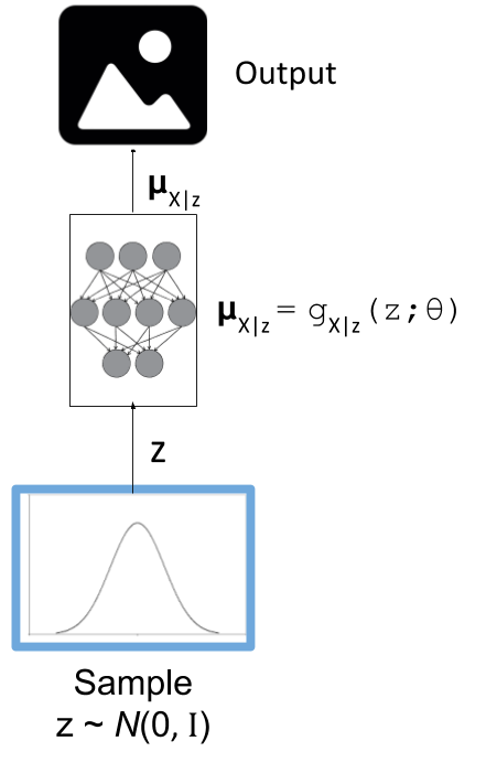
Figure 5: The generative model component of a variational autoencoder in test mode.

Figure 5 shows our generative model. To generate a new observation, all we have to do is sample from our isotropic normal distribution (our prior for our latent variables), and then run it through our neural network. The network should have learned how to transform our latent variables into the mean of what our training data looks like 2.

Note, that our network now only outputs the mean of our generative output, we can additionally sample from our actual output distribution if we sample a normal distribution with this mean. In most cases, the mean is probably what we want though (e.g. when generating an image, the mean values are just the values for the pixels).

4. A Basic Example: MNIST Variational Autoencoder

The nice thing about many of these modern ML techniques is that implementations are widely available. I put together a notebook that uses Keras to build a variational autoencoder 3. The code is from the Keras convolutional variational autoencoder example and I just made some small changes to the parameters. I also added some annotations that make reference to the things we discussed in this post.

Figure 6 shows a sample of the digits I was able to generate with 64 latent variables in the above Keras example.

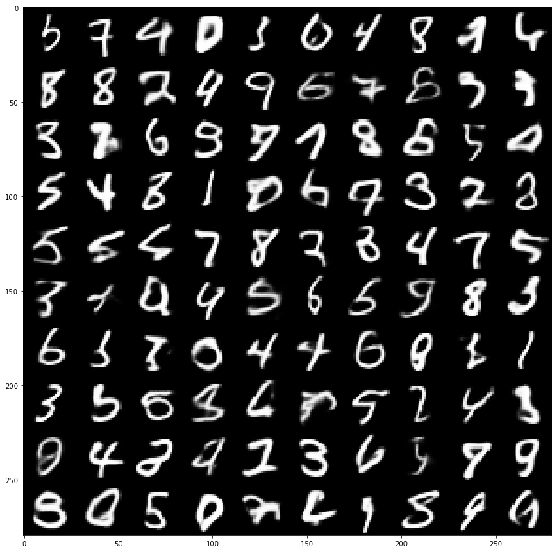
Figure 6: MNIST digits generated from a variational autoencoder model.

Not the prettiest hand writing =) We definitely got some decent looking digits but also some really weird ones. Usually the explanation for the weird ones are that they're in between two digits or two styles of writing the same digit (or maybe I didn't train the network well?). An example might be the top left digit. Is it a "3", "5" or "6"? Kind of hard to tell.

Anyways take a look at the notebook, I find it really interesting to see the connection between theory and implementation. It's often that you see an implementation and it's very difficult to reverse-engineer it back to the theory because of all the simplifications that have been done. Hopefully this post and the accompanying notebook will help.

Conclusion

Variational autoencoders are such a cool idea: it's a full blown probabilistic latent variable model which you don't need explicitly specify! On top of that, it builds on top of modern machine learning techniques, meaning that it's also quite scalable to large datasets (if you have a GPU). I'm a big fan of probabilistic models but an even bigger fan of practical things, which is why I'm so enamoured with the idea of these variational techniques in ML. I plan on continuing in this direction of exploring more of these techniques in ML that have a solid basis in probability. Look out for future posts!

Further Reading

• Previous Posts: Variational Bayes and The Mean-Field Approximation, Variational Calculus

• Wikipedia: Variational Bayesian methods, Generative Models, Autoencoders, Kullback-Leibler divergence, Inverse transform sampling

• "Tutorial on Variational Autoencoders", Carl Doersch, https://arxiv.org/abs/1606.05908

1

Said another way, the posterior distribution for each sample \(p(z|X=x_i)\) has some distinctive shape that is probably very different from the prior \(p(z)\). If we sample any given \(z_m\sim Z\) (which has distribution \(p(z)\)), then most of those samples will have low \(p(Z=z_m|X=x_i)\) because the distributions have vastly different shapes. This implies that, \(p(X=x_i|Z=z_m)\) (recall Bayes theorem) will also be low, which implies little contribution to our likelihood in Equation 7.

2

If you find this a bit confusing, here's another explanation. The only reason we did all the work on the "encoder" part was to generate a good distribution for \(z|X\). That is given an \(x_i\), find the likely \(z\) values. However, we made sure that when we average over all the \(X\) observations, our average \(z\) values would still match our prior \(p(z)\) isotropic normal distribution via the KL divergence. That means, sampling for our isotropic normal distribution should still give us likely values for \(z\).

3

I initially just tried to use this example with just my CPU but it was painfully slow (~ 5+ min/epoch). So I embarked on a multi-week journey to buy a modern GPU, re-build my computer and dual-boot Linux (vs. using a virtual machine). The speed-up was quite dramatic, now it's around ~15 secs/epoch.