Universal ResNet: The One-Neuron Approximator

"In theory, theory and practice are the same. In practice, they are not."

I read a very interesting paper titled ResNet with one-neuron hidden layers is a Universal Approximator by Lin and Jegelka [1]. The paper describes a simplified Residual Network as a universal approximator, giving some theoretical backing to the wildly successful ResNet architecture. In this post, I'm going to talk about this paper and a few of the related universal approximation theorems for neural networks. Instead of going through all the theoretical stuff, I'm simply going introduce some theorems and play around with some toy datasets to see if we can get close to the theoretical limits.

(You might also want to checkout my previous post where I played around with ResNets: Residual Networks)

Universal Approximation Theorems

The OG Universal Approximation Theorem

The Universal Approximation Theorem (1989) is one of the most well known (and often incorrectly used) theorems when it comes to neural networks. It's probably because neural networks don't have as much theoretical depth as other techniques so people feel like they have to give some weight to its spectacular empirical results. I'll paraphrase the theorem here (if you're really interested in the math click on the Wikipedia link):

The universal approximation theorem states that a feed-forward network with a single hidden layer containing a finite number of neurons can approximate functions on compact sets on \(\mathbb{R}^n\), under mild assumptions of the activation function (non-constant, monotonically-increasing, continuous).

The implications is theoretically we can approximate any function just by arbitrarily increasing the width of a single hidden layer.

For me, this theorem doesn't strike me as all that insightful (or useful). First, in practice we never arbitrarily make the width of a neural network really wide, never mind having a single hidden layer. Second, it seems intuitive that this might be the case doesn't it? If we think about approximating a function with an arbitrary number of piece-wise linear functions, then we should be able to approximate most well-behaved functions (that's basically how integration works). Similarly, if we have a neuron for each "piece" of the function, we should intuitively be able to approximate it to any degree (although I'm sure the actual proof is much more complicated and elegant).

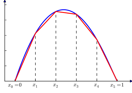
Figure 1: If we can approximate functions with an arbitrary number of piece-wise linear functions, why can't we do it with an arbitrary number of hidden units? (source: Wikipedia)

So practically, there isn't much that's interesting about this (basic) version of the theorem. And definitely, people should stop quoting it as if it somehow "proved" something.

Universal Approximation Theorem for Width-Bounded ReLU Networks

A much more interesting result for neural networks is a universal approximation theorem for width-bounded neural networks published recently (2017) from [2]:

Let \(n\) denotes the input dimension, we show that width-\((n + 4)\) ReLU networks can approximate any Lebesgue integrable function on n-dimensional space with respect to L1 distance.

Additionally, except for a negligible set, most functions cannot be approximated by a ReLU network of width at most \(n\).

So basically if you have just 4 extra neurons in each layer and arbitrary number of hidden layers, you can approximate any Lebesque integrable function (which are most functions). This result is very interesting because this is starting to look like a feed-forward network that we might build. Just take the number of inputs, add 4, and then make a bunch of hidden layers of that size. Of course, training this is another story, which we'll see below. The negative result is also very interesting. We need some extra width or else we'll never be able to approximate anything. There are also a whole bunch of other results on neural networks that have been proven. See the references from [1] and [2] if you're interested.

Universal Approximation Theorem for The One-Neuron ResNet

ResNet is a neural network architecture that contains a "residual connection". Basically, it provides a shortcut from layer \(i\) merging it with addition to layer \(i+k\) for some constant \(k\). In between, you can do all kinds of interesting things such as have multiple layers, increase or bottleneck the width, but the important thing is that the input width of layer \(i\) is the same as the output width of layer \(i+k\). Figure 2 shows a simplified ResNet architecture where the "in between" transformation is a single neuron.

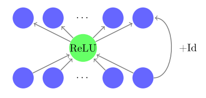
Figure 2: The basic residual block with one neuron per hidden layer (source: [1])

Note that through this ResNet block there are two paths: one that goes through a bottleneck of a single neuron, and one that is the identity function. The outputs then get added together at the end. Writing out the expression of the function, we have our ResNet block \(\mathcal{R}_i(x)\) and our final network \(Y(x)\):

where \(\bf U\) is \(d \text{x} 1\) weight matrix, \(\bf V\) is \(1\text{x}d\) weight matrix, and \(b\) is a learnable constant.

Given the above ResNet architecture, the universal approximation theorem from [1] states:

ResNet with one single neuron per hidden layer is enough to provide universal approximation for any Lebesgue-integrable function as the depth goes to infinity.

This is a pretty surprising statement! Remember, this architecture's only non-linear element is a bottleneck with a single neuron! However, this theorem somehow gives credibility to the power of Residual Networks because even with a single neuron it is powerful enough to represent any function.

Experiments

In this section I play around with a few different network architectures relating to the theorems above to see how they would perform. You can see my work in this notebook on GitHub.

I generated three toy datasets labelled "easy", "medium", "hard" with two input variables \(x_1, x_2\), and a single binary label. Each dataset used the same 300 \((x_1, x_2)\) input points but had different predicates of increasing complexity. Figure 3 shows the three datasets.

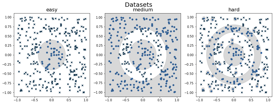
Figure 3: Plot of "easy", "medium" and "hard" datasets. The shaded region indicates where the generating function should be a "1". The "x"s represent "0"s and the dots represent "1"s. Notice the "hard" dataset has a bunch of spurious "1"s that are randomly placed on the grid.

First, let's take a look at the different architectures that I ran. All the experiments use a softmax output layer with a binary crossentropy loss.

• Resnet: Stacking the above ResNet block (figure 2) with a width of 2 (same as the input).

• Dense (W=2, W=6): Fully connected dense layers with a width of either 2 (size of inputs) or 6 (size of inputs + 4 from the universal theorem above) with ReLU activations.

• Single Dense with Variable Width: A single hidden layer but changing the width (OG universal theorem) with ReLU activations.

I varied depths of the first two architectures varied from 5, 10, and 40. The width of the last architecture varies from 5, 10, 40, 100, and 300. For each combination, I ran 5 experiments and report the mean and standard deviation of accuracy on the training data (no testing set here since we're trying to see if it can approximate samples from the underlying function). Bolded results show the best run for each dataset. The overall results are shown in Table 1 and Table 2, while Appendix A shows figures plotting the best run of each configuration.

Table 1: ResNet vs. Dense (W=2, 6) with varying depths on Easy, Medium and Hard datasets.

We can see in Table 1 that ResNet has pretty consistent performance. As we increase the depth, it's able to successfully translate the increased capacity into accuracy gains. Not only that, it shows the best best performance in the easy and hard datasets, while being pretty close on the medium one. The fact that we are able to train a network so deep shows the uncanny ability of ResNet architectures to train deep networks (as compared to the dense layers). So the ResNet universal approximation theorem for ResNet seems to be holding up somewhat.

For the dense networks with width=2, it is totally incapable of learning anything useful. The accuracies reported are actually just the underlying ratio of positive to negative labels where it pretty much just learned the constant function (see figures in Appendix A). This confirms the negative result of the width bounded universal approximation theorem.

At width=6, the dense network shows more mixed results. It performs quite well at depths 5 and 10, even producing the best result on the medium dataset at depth=5. However, it totally breaks down at depth 40. This is most likely due to the difficulty of fitting really deep networks. An important lesson: theoretical results don't always translate into practical ones. (We probably could have helped this along by adding some normalization to fit the deep networks. I did add do one trial with batch normalization but the results didn't change much.)

Table 2: Dense with a single hidden layer and varying width on Easy, Medium and Hard datasets.

Taking a look at similar results with a single hidden layer architecture in Table 2, we see that the original universal approximation theorem shows more consistent results. Each increase in width is better than the previous except at W=300 where it performs pretty close to the width below it. It performs on-par with the above architectures except on the hard where it performs slightly worse. However, we can see the results across the board are much more consistent (smaller standard deviation). This indicates that the single hidden layer is also the easier to fit (no vanishing gradients). However, it's also been shown to be very inefficient -- you might need a non-linear (exponential?) number of units before you can approximate something. It turns out that these datasets aren't that hard so 100 or so hidden units will do.

Conclusion

Definitely a shorter post than my previous few. Although like many theoretical results these ones aren't too practical, but I thought this result was so interesting because of the strong empirical evidence in favour of ResNet architectures. Many results in deep learning don't have great theoretical foundations, so it's so nice to see a result for one of big ideas in this area. My next post will likely be a shorter one too with another cute idea that I've read about recently. Stay tuned!

Further Reading

• Previous posts: Residual Networks

• Wikipedia: Universal Approximation Theorem

• [1] ResNet with one-neuron hidden layers is a Universal Approximator, Hongzhou Lin, Stefanie Jegelka

• [2] The Expressive Power of Neural Networks: A View from the Width Zhou Lu, Hongming Pu, Feicheng Wang, Zhiqiang Hu, Liwei Wang

Appendix A: Figures for Experiments

The figures below show the best run out of the five runs for each of the given experiments. So the accuracies are at the top of the range and do not match the averages in Table 1 and 2.

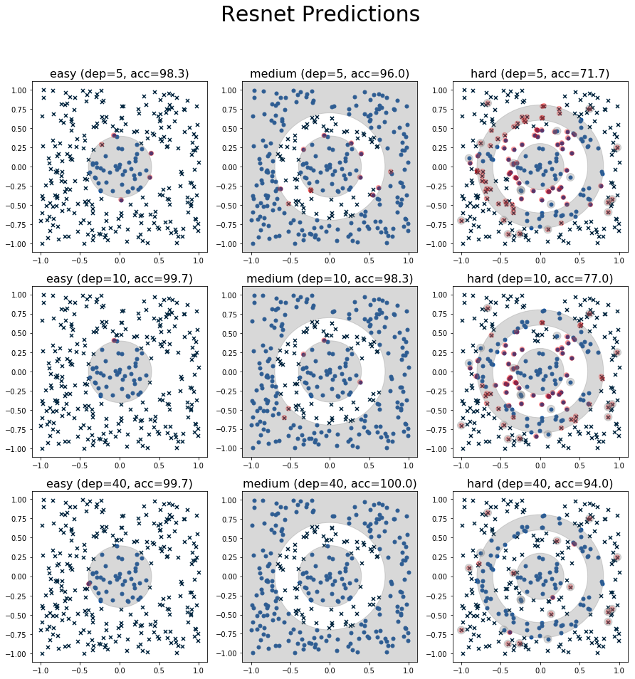
Figure 3: Plot of predictions from the ResNet architecture.

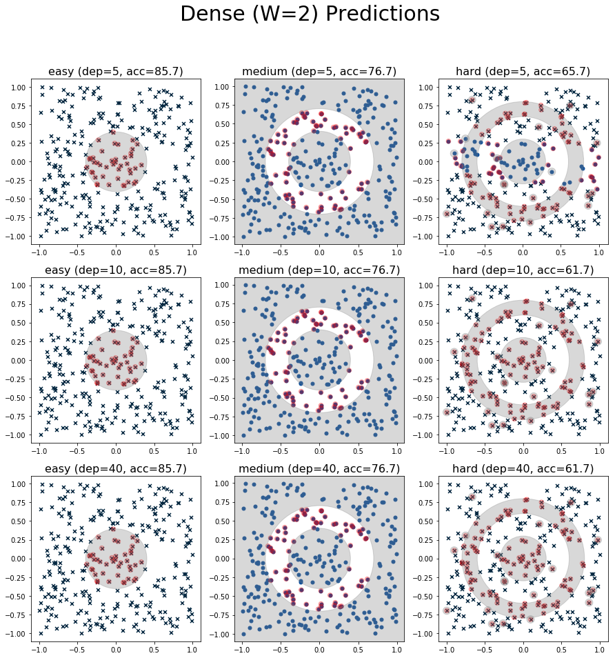
Figure 4: Plot of predictions from the Dense (W=2) architecture.

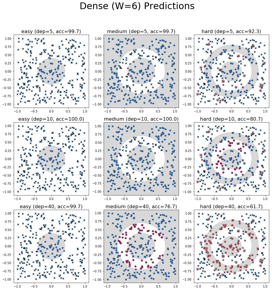
Figure 5: Plot of predictions from the Dense (W=6) architecture.

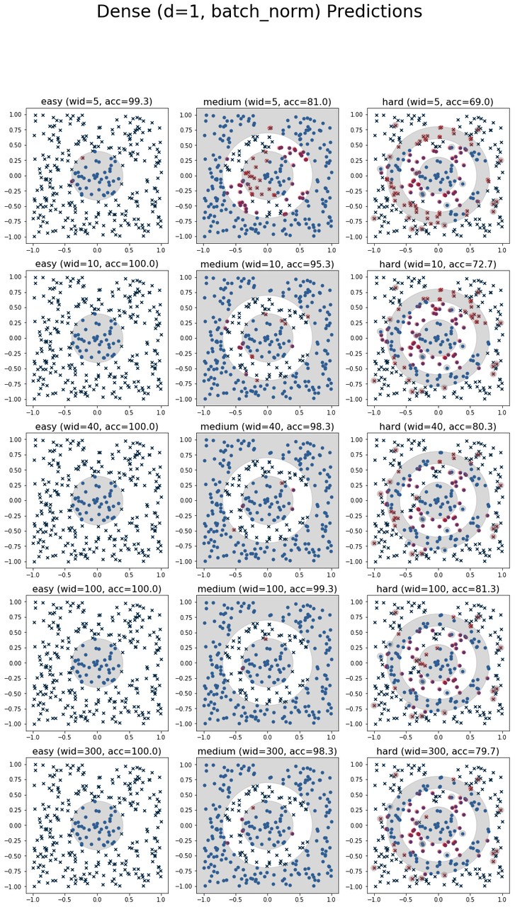
Figure 6: Plot of predictions from the Single Dense architecture.