Residual Networks

Brian Keng

2018-02-18 13:55

Taking a small break from some of the heavier math, I thought I'd write a post (aka learn more about) a very popular neural network architecture called Residual Networks aka ResNet. This architecture is being very widely used because it's so simple yet so powerful at the same time. The architecture's performance is due its ability to add hundreds of layers (talk about deep learning!) without degrading performance or adding difficulty to training. I really like these types of robust advances where it doesn't require fiddling with all sorts of hyper-parameters to make it work. Anyways, I'll introduce the idea and show an implementation of ResNet on a few runs of a variational autoencoder that I put together on the CIFAR10 dataset.

More layers, more problems?

In the early days, a 4+ layer network was considered deep, and rightly so! It just wasn't possible to train mostly because of problems such as vanishing/exploding gradients caused in part by the sigmoid or tanh activation functions. Of course, nowadays there are things like weight initialization, batch normalization, and various improved activation functions (e.g. ReLU, ELU, etc.) that have more or less overcome many of these issues (see original paper [1] for a bunch of the relevant references).

However, once we started to be able to train more layers, it seemed that a new type of problem started happening called degradation. After a certain point, adding more layers to a network caused it to have worse performance. Moreover, it was clear that it was not an overfitting issue because training error increased (you'd expect training error to decrease but testing error to increase in an overfitting scenario). It doesn't quite make sense why adding more layers would cause problems.

Theoretically, if there was some magical optimal number of layers, you would intuitively just expect any additional layers to just learn the identity mapping, essentially learning a "null-op". However, empirically this is not what is observed where performance is usually worse. This insight leads to the idea of residual networks.

Residual Learning

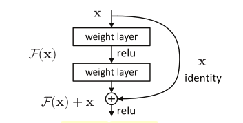
The big idea is this: why not explicitly allow a "shortcut" connection and let the network figure out what to use? Figure 1 shows this a bit more clearly.

Figure 1: The basic ResNet building block (source: [1])

The basic idea is simply to add an identify connection every few layers that adds the source of the block, \(\bf x\), to the output of the block \(\mathcal{F}({\bf x})\), resulting in the final output of \(\mathcal{H}({\bf x}) := \mathcal{F}({\bf x}) + {\bf x}\). The name "residual networks" comes from the fact, we're actually learning \(\mathcal{F}({\bf x}) = \mathcal{H}({\bf x}) - {\bf x}\), the "residual" of what's left over when you subtract input from output.

As with many of these architectures, there's no mathematical proof of why things work but there are a few hypotheses. First, it's pretty intuitive that if a neural net can learn \(\mathcal{H}({\bf x})\), it can surely learn the residual \(\mathcal{F}({\bf x}) - x\). Second, even though theoretically they are solving the same problem, the residual may be an easier function to fit, which is what we actually see in practice. Third, more layers can potentially help model more complex functions with the assumption being that you are able to train the deeper network in the first place.

One really nice thing about these shortcuts is that we don't add any new parameters! We simply add an extra addition operation in the computational graph allowing the network to be trained in exactly the same way as the non-ResNet graph. It also has the added benefit of being relatively easy to train even though this identity connection architecture is most likely not the theoretical optimal point for any given problem.

One thing to note is that the dimensions of \(\bf x\) and \(\mathcal{F}({\bf x})\) have to match, otherwise we can do a linear projection of \({\bf x}\) onto the dimension like so:

\begin{equation*} \mathcal{H}({\bf x}) := \mathcal{F}({\bf x}) + W_s{\bf x} \tag{1} \end{equation*}

where \(W_x\) is a weight matrix that can be learned.

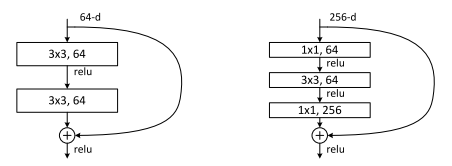
For convolutional networks, [1] describes two types of building blocks reproduced in Figure 2. The left block is a simple translation of Figure 1 except with convolutional layers. The right block uses a bottleneck design using three successive convolutional layers. Each layer has stride one, meaning the input and output pixel dimensions are the same, the main difference is the filter dimensions which are 64, 64, 256 respectively in the diagram (these are just examples of numbers). So from a 256 dimension filter input, we reduce it down to 64 in the first 1x1 and 3x3 layers, and the scale it back up to 256, hence the term bottleneck.

Figure 2: Two Types of Convolutional ResNet building blocks (source: [1])

Once you have these building blocks, all you do is just stack them sequentially! You can stack dozens of them without much problem. There are also a few additional details when building a full ResNet implementation. The one I will mention is that every few blocks, you'll want to scale down (or up in the case of a decoder) the image dimension. Take a look at the implementation I used (which is originally from Keras) and it should make more sense.

Experiments

The experiments in [1] are quite extensive, so I'd encourage you to take a look. In fact, the experiments are basically the entire paper because the idea is so simple. They are able to train networks with over a 1000 layers (although that one didn't perform the best). It's quite convincing and the overall trend is that very deep nets (100+ layers) perform better than shallower ones (20-50 layers) as well as other state of the art architectures.

So since I already had a lot of code around for variational autoencoders, I decided to see ResNet would help at all. Using a vanilla autoencoder (diagonal Gaussian latent variables) on the CIFAR10 dataset didn't produce very good results from some previous experience (see post on Semi-supervised Learning with Variational Autoencoders). One thing I was wondering is if adding a high capacity encoder/decoder network like ResNet would benefit the model performance.

You can find my implementation here on Github.

CIFAR10 VAE Results

For these experiments, I basically used the ResNet implementation from Keras with a few modifications such as supporting transposed convolutions for the decoder. It should be pretty straight forward to see in the code if you're curious. The results for the different depths of ResNet are in Table 1.

Table 1: CIFAR10 VAE Results
Depth	Training Time (hrs)	Training Loss	Validation Loss
28	79.2	1790.4	1794.7
40	61.9	1787.5	1795.7
70	80.0	1784.8	1799.0
100	164.7	1782.3	1804.0

As you can see not much has changed in terms of model performance between the different runs but look at those depths! The training loss seems to improve a bit but the validation loss seems to get slightly worse. Of course the difference is so small you can't really make any conclusions. All I really conclude from this is that this vanilla VAE setup isn't powerful enough to represent the CIFAR10 dataset 1. Another thing to note is that visually the generated images from each of the runs all look similarly blurry.

I used an early stopping condition for each run where it would stop if the validation loss hadn't improved for 50 runs. Interestingly when looking at runtime on my meager GTX1070, it seems that even deeper nets can "converge" faster. What we can conclude from this is that making the net significantly deeper didn't really hurt performance at all. We didn't have any problems training, nor did it really increase the run-time all that much except when we went much deeper. We didn't get the big benefits of using deeper nets in this case (probably a limitation of the VAE), but ResNet is really robust!

Implementation Notes

Here are some implementation notes:

I used the Keras ResNet identity_block and conv_block as a base. Modifying the latter to also support transposed convolutions.
I finally took a bit of time to figure out how to use nested Model's in Keras. So basically I just have to make the encoder/decoder Model once, build the VAE by nesting those two Model's to build a VAE Model. This makes it much easier to build the "generator"/decoder by just instantiating the encoder Model. I actually tried doing this a while back but came across some errors, so I just decided to duplicate code by recreating a new flat generator Model with the same layers. This time it was too hard to do because of how the ResNet blocks are instantiated so I took the time to figure it out. I forgot exactly what error I was getting but at least you can look at the code I put together to see an example of it working.
The other "smarter" thing that I did was I wrote a script to run the notebook through command line. This is great because when I'm just messing around I want to be able to see things in a UI but I also want to be able to batch run things (I only have 1 GPU after all). This really allowed me to have the best of both worlds. I'll just mention a few specific tricks I used:
- Any variables I wanted to be able to modify from command-line I had to add something like os.environ.get('LATENT_DIM', 256), which allows you to read command-line environment variables.
- In my run script, I had to define a CMDLINE var to not run certain UI-specific code such as TQDMNotebookCallback(), which is a delight to have in the UI but causes issues when running from the command line.
- In my run script, I used the Jupyter functionality to run from command line. The main thing to add is --ExecutePreprocessor.timeout=-1 so that it will not timeout when you're doing the actual fitting (it has a default of something like 10 mins if a cell takes too long).

Conclusion

So there you have it, a quick introduction to ResNet in all its glory. I don't know about you but it really gives me an adrenaline rush training a 100 layer deep neural network! So cool! Of course, I also enjoy learning about differential geometry on my vacation (future post), so I guess I have a special personality.

This post definitely has much less math that my recent stuff but rest assured that I have much more math heavy posts coming up. I have at least four topics I want to investigate and write about, I just need to find some time to work on them. Expect the usual slow trickle instead of a flood. See you next time!