Manifolds: A Gentle Introduction

Brian Keng

2018-04-17 06:24

Following up on the math-y stuff from my last post, I'm going to be taking a look at another concept that pops up in ML: manifolds. It is most well-known in ML for its use in the manifold hypothesis. Manifolds belong to the branches of mathematics of topology and differential geometry. I'll be focusing more on the study of manifolds from the latter category, which fortunately is a bit less abstract, more well behaved, and more intuitive than the former. As usual, I'll go through some intuition, definitions, and examples to help clarify the ideas without going into too much depth or formalities. I hope you mani-like it!

Manifolds

The first place most ML people hear about this term is in the manifold hypothesis:

The manifold hypothesis is that real-world high dimensional data (such as images) lie on low-dimensional manifolds embedded in the high-dimensional space.

The main idea here is that even though our real-world data is high-dimensional, there is actually some lower-dimensional representation. For example, all "cat images" might lie on a lower-dimensional manifold compared to say their original 256x256x3 image dimensions. This makes sense because we are empirically able to the learn these things in a capacity limited neural network. Otherwise learning an arbitrary 256x256x3 function would be intractable.

Okay, that's all well and good, but that still doesn't answer the question: what is a manifold? The abstract definition from topology is well... abstract. So I won't go into all the technical details (also because I'm not very qualified to do so), but we'll see that the differential and Riemannian manifolds are surprisingly intuitive (in low dimensions at least) once you get the hang (or should I say twist) of it.

(Note: You should check out [1] and [2], which are great YouTube playlists for understanding these topics. [2] especially is just as good (or better) than a lecture at a university. I used both of these playlists extensively to write this post.)

Circles and Spheres as Manifolds

A manifold is a topological space that "locally" resembles Euclidean space. This obviously doesn't mean much unless you've studied topology. An intuitive (but not exactly correct) way to think about it is taking a geometric object from \(\mathbb{R}^k\) and trying to "fit" it into \(\mathbb{R}^n, n>k\). Let's take a first example, a line segment, which is obviously one dimensional.

One way to embed a line in two dimensions is to "wrap" it around into a circle, shown in Figure 1. Each arc of the circle locally looks closer to a line segment, and if you take an infinitesimal arc, it will "locally" resemble a one dimensional line segment.

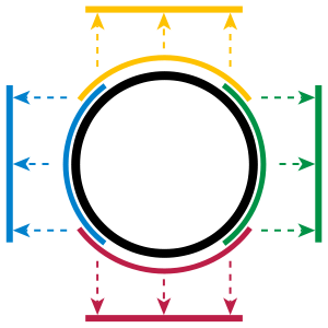
Figure 1: A circle is a one-dimensional manifold embedded in two dimensions where each arc of the circle locally resembles a line segment (source: Wikipedia).

Of course, there is a much more precise definition from topology in which a manifold is defined as a special set that is locally homeomorphic to Euclidean space. A homeomorphism is a special kind of continuous one-to-one and onto mapping that preserves topological properties. The definition is quite abstract because the definition says a (topological) manifold is just a special kind of set without any explicit reference of how it can be viewed as a geometric object. We'll take a closer look at this a bit below, but for now, let's focus on the big idea.

Actually any "closed" loop in one dimension is a manifold because you can imagine "wrapping" it around into the right shape. Another way to think about it (from the formal definition) is that from a line (segment), you can find a continuous one-to-one mapping to a closed loop. An interesting point is that figure "8" is not a manifold because the crossing point does not locally resemble a line segment.

These closed loop manifolds are the easiest 1D manifolds to think about but there are other weird cases too shown in Figure 2. As you can see, we can have a variety of different shapes. The big idea is that we can also have "open ended" curves that extend out to infinity, which are natural mappings to a one dimensional line.

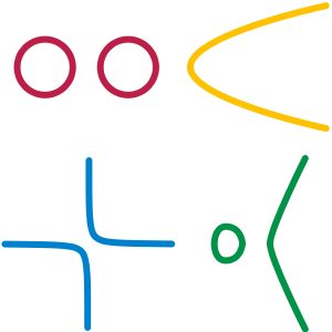
Figure 2: Circles, parabolas, hyperbolas and cubic curves are all 1D Manifolds. Note: the four different colours are all on separate axes and extend out to infinity if it has an open end (source: Wikipedia).

Let's now move onto 2D manifolds. The simplest one is a sphere. You can imagine each infinitesimal patch of the sphere locally resembles a 2D Euclidean plane. Similarly, any 2D surface (including a plane) that doesn't self-intersect is also a 2D manifold. Figure 3 shows some examples.

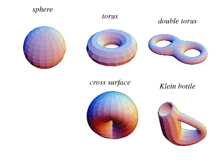
Figure 3: Non-intersecting closed surfaces in \(\mathbb{R}^3\) are examples of 2D manifolds such as a sphere, torus, double torus, cross surfaces and Klein bottle (source: Wolfram).

For these examples, you can imagine that each point on these manifolds locally resembles a 2D plane. This best analogy is Earth. We know that the Earth is round but when we stand in a field it looks flat. We can of course have higher dimension manifolds embedded in even larger dimension Euclidean spaces but you can't really visualize them. Abstract math is rarely easy to reason about in higher dimensions.

Hopefully after seeing all these examples, you've developed some intuition around manifolds. In the next section, we'll head back to the math with some differential geometry.

A (slightly) More Formal Look at Manifolds

Now that we have some intuition, let's take a first look at the formal definition of (topological) manifolds, which I took from [1]:

An n-dimensional topological manifold \(M\) is a topological Hausdorff space with a countable base which is locally homeomorphic to \(\mathbb{R}^n\). This means that for every point \(p\) in \(M\) there is an open neighbourhood \(U\) of \(p\) and a homeomorphism \(\varphi: U \rightarrow V\) which maps the set \(U\) onto an open set \(V \subset \mathbb{R}^n\). Additionally:

The mapping \(\varphi: U \rightarrow V\) is called a chart or coordinate system.

The set \(U\) is the domain or local coordinate neighbourhood of the chart.

The image of the point \(p \in U\), denoted by \(\varphi(p) \in \mathbb{R}^n\), is called the coordinates or local coordinates of \(p\) in the chart.

A set of charts, \(\{\varphi_\alpha | \alpha \in \mathbb{N}\}\), with domains \(U_\alpha\) is called the atlas of M, if \(\bigcup\limits_{\alpha \in \mathbb{N}} U_\alpha = M\).

This definition is hard to understand especially because a Hausdorff space is never defined. That's not too important because we're not going to go into the topological formalities, the most important parts are the new terminology, which thankfully have an intuitive interpretation. Let's take a look at Figure 4, which should clear up some of the ideas.

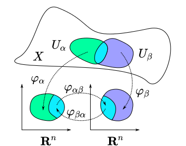
Figure 4: Two intersecting patches (green and purple with cyan/teal as the intersection) on a manifold with different charts (continuous 1-1 mappings) to \(\mathbb{R}^n\) Euclidean space. Notice that the intersection of the patches have a smooth 1-1 mapping in \(\mathbb{R}^n\) Euclidean space, making it a differential manifold (source: Wikipedia).

First of all our manifold in this case is \(X\), which we can imagine is embedded in some high dimension \(n+k\). We have two different "patches" or domains (or local coordinate neighbourhoods) defined by \(U_\alpha\) (green) and \(U_\beta\) (purple) in \(X\). Since it's a manifold, we know that each point locally has a mapping to a lower dimensional Euclidean space (say \(\mathbb{R}^n\)) via \(\varphi\), our chart or coordinate system. If we take a point \(p\) in our domain, and map it into the lower dimensional Euclidean space, the mapped point is called the coordinate or local coordinate of \(p\) in our chart. Finally, if we have a bunch of charts whose domains exactly spans the entire manifold, then this is called an atlas.

The best analogy for all of this is really just geography. I've never really studied geography beyond grade school but I'm guessing you have similar terminology such as charts, coordinate systems, and atlases. The ideas are, on the surface, similar. However, I'd probably still stick with Figure 4, which is much more accurate.

Manifolds: All About Mapping

Wrapping your head around manifolds can be sometimes be hard because of all the symbols. The key thing to remember is that manifolds are all about mappings. Mapping from the manifold to a local coordinate system in Euclidean space using a chart; mapping from one local coordinate system to another coordinate system; and later on we'll also see mapping a curve or function on a manifold to a local coordinate too. Sometimes we'll do one "hop" (e.g. manifold to local coordinates), or multiple "hops" (parameter of a curve to location on a manifold to local coordinates). And since most of our mappings are 1-1 we can "hop" back and forth as we please to get the mapping we want. So make sure you are comfortable with how to do these "hops" which are nothing more than simple function compositions.

Figure 4 also has another mapping between the intersecting parts of \(U_\alpha\) and \(U_\beta\) in their respective chart coordinates called a transition map, given by \(\varphi_{\alpha\beta} = \varphi_\beta \circ \varphi_\alpha^{-1}\) and \(\phi_{\beta\alpha}=\varphi_\alpha \circ \varphi_\beta^{-1}\) (their domain is restricted to either \(\varphi_\alpha(U_\alpha \cap U_\beta)\) or \(\varphi_\beta(U_\alpha \cap U_\beta)\), respectively).

These transition functions are important because depending on their differentiability, they define a new class of differentiable manifolds (denoted by \(C^k\) if they are k-times continuously differentiable). The most important one for our conversation being transition maps that are infinitely differentiable, which we call smooth manifolds.

The motivation here is that once we have smooth manifolds, we can do a bunch of nice things like calculus. Remember, once we have smooth mappings to lower dimensional Euclidean space, things are a lot easier to analyze. Performing analysis on a manifold embedded in a high dimensional space could be a major pain in the butt, but analysis in a lower-dimensional Euclidean space is easy (relatively)!

Example 1: Euclidean Space is a Manifold

Standard Euclidean space in \(\mathbb{R}^n\) is, of course, a manifold itself. It requires a single chart that is just the identity function, which also makes up its atlas. We'll see below that many of concepts we've been learned in Euclidean space have analogues when discussing manifolds.

Example 2: A 1D Manifold with Multiple Charts

Let's take pretty much the simplest example we can think of: a circle.

If we use polar coordinates, the unit circle can be parameterized with \(r=1\) and \(\theta\).

The unit circle is a 1D manifold \(M\), so it should be able to map to \(\mathbb{R}\). We might be tempted to just have a simple chart mapping such as \(\varphi(r, \theta) = \theta\) but because \(\theta\) is a multi-valued we need to restrict the domain. Further, we'll need more than one chart mapping because a chart can only work on an open set (the analogue to an open interval, i.e. we can't use \([0, 2\pi)\)).

We can create four charts (or mappings) as in Figure 1, that have the form \(M \rightarrow \mathbb{R}\):

\begin{align*} \varphi_1(r, \theta) &= \theta && \theta \in (-\frac{\pi}{3}, \frac{\pi}{3}) \\ \varphi_2(r, \theta) &= \theta && \theta \in (\frac{\pi}{6}, \frac{5\pi}{6}) \\ \varphi_3(r, \theta) &= \theta && \theta \in (\frac{2\pi}{3}, \frac{4\pi}{3}) \\ \varphi_4(r, \theta) &= \theta && \theta \in (\frac{7\pi}{6}, \frac{11\pi}{6}) \\ \tag{1} \end{align*}

Notice that there is overlap in \(\theta\) between the charts where each one has an open set (i.e. the domain) on the original circle. \({\varphi_1, \varphi_2, \varphi_3, \varphi_4}\) together form an atlas for \(M\) because their domains span the entirety of the manifold.

We can also find other charts to map the unit circle. Let's take a look at another construction using standard Euclidean coordinates and a stereographic projection. Figure 5 shows a picture of this construction.

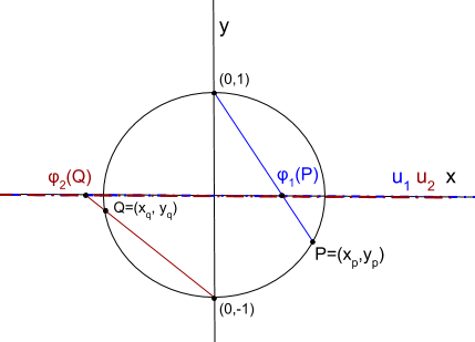
Figure 5: A construction of charts on a 1D circle manifold.

We can define two charts by taking either the "north" or "south" pole of the circle, finding any other point on the circle and projecting the line segment onto the x-axis. This provides the mapping from a point on the manifold to \(\mathbb{R}^1\). The "north" pole point is visualized in blue, while the "south" pole point is visualized in burgundy. Note: the local coordinates for the charts are different. The same point on the circle mapped via the two charts do not map to the same point in \(\mathbb{R}^1\).

Using the "north" pole point, for any other given point \(p=(x,y)\) on the circle, we can find where it intersects the x-axis via similar triangles (the radius of the circle is 1, \(\frac{\text{adjacent}}{\text{opposite}}\)):

\begin{equation*} u_1 := \varphi_1(p) = \frac{\varphi_1(p)}{1} = \frac{x_p}{1 - y_p} \tag{2} \end{equation*}

This defines a mapping for every point on the circle except the "north" pole. Similarly, we can define the same mapping for the "south" pole for any point on the circle \(q\) (except the "south" pole):

\begin{equation*} u_2 := \varphi_2(q) = \frac{\varphi_2(q)}{1} = \frac{x_q}{1 + y_q} \tag{3} \end{equation*}

Together, \({\varphi_1, \varphi_2}\) make up an atlas for \(M\). Since charts are 1-1, we can find the inverse mapping between the manifold and local coordinates as well (using the fact that \(x^2 + y^2=1\)):

\begin{align*} x_p &= \frac{2u_1}{u_1^2+1}, &y_p = \frac{u_1^2-1}{u_1^2+1} \\ x_q &= \frac{2u_2}{u_2^2+1}, &y_q = \frac{1-u_2^2}{u_2^2+1} \\ \tag{4} \end{align*}

Finally, we can find the transition map \(\varphi_{\alpha\beta}\) as:

\begin{align*} u_2 &= \varphi_{\alpha\beta}(u_1) \\ &= \varphi_2 \circ \varphi_1^{-1}(u_1) \\ &= \varphi_2(\varphi_1^{-1}(u_1)) \\ &= \varphi_2\big((\frac{2u_1}{u_1^2+1}, \frac{u_1^2-1}{u_1^2+1})\big) \\ &= \frac{\frac{2u_1}{u_1^2+1}}{1 + \frac{u_1^2-1}{u_1^2+1}} \\ &= \frac{1}{u_1} \\ \tag{5} \end{align*}

which is only defined for the points in the intersection (i.e. all points on the circle except the "north" and "south" pole).

Example 3: Stereographic Projections for \(S^n\)

As you might have guessed, we can perform the same stereographic projection for \(S^2\) as well. Figure 6 shows a visualization (never mind the different notation, I used a drawing from Wikipedia instead of trying to make my own :p).

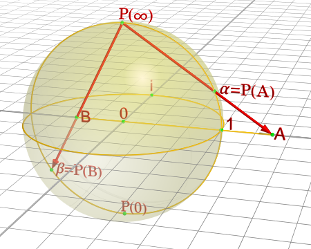
Figure 6: A construction of charts on a 2D sphere (source: Wikipedia).

In a similar way, we can pick a point, draw a line that intersects any other point on the sphere, and project it out to the \(z=0\) (2D) plane. This chart can cover every point except the starting point. Using two charts each with a point (e.g. "north" and "south" pole), we can create an atlas that covers every point on the sphere.

In general an n-dimensional sphere is a manifold of \(n\) dimensions and is given the name \(S^n\). So a circle is a 1-dimensional sphere, a "normal" sphere is a 2-dimensional sphere, and a n-dimensional sphere can be embedded in (n+1)-dimensional Euclidean space where each point is equidistant to the origin.

This projection can generalized for \(S^n\) using the same method:

Pick an arbitrary focal point on the sphere (not on the hyperplane you are projecting to) e.g. the "north" pole \(p_N = (0, \ldots, 0,1)\).
Project a line from the focal point to any other point on the hypersphere.
Pick a plane that intersects at the "equator" relative to the focal point. e.g. For the "north" pole focal point, the plane given by the first \(n\) coordinates (remember the \(S^n\) has n+1 coordinates because it's embedded in \(\mathbb{R}^{n+1}\)).

From this, we can derive similar formulas (using the same similar triangle argument) as the previous example. Using the north pole as an example to any point \(p =({\bf x}, z) \in S^n\) on the hypersphere, and the hyperplane given by \(z=0\), we can get the projected point \(({\bf u_N}, 0)\) using the following equations:

\begin{align*} {\bf u_N} := \varphi_N(p) = \frac{\bf x}{1 - z} \\ {\bf x} = \frac{2{\bf u_N}}{|{\bf u_N}|^2 + 1} \\ z = \frac{|{\bf u_N}|^2 - 1}{|{\bf u_N}|^2 + 1} \\ \tag{6} \end{align*}

for vectors \({\bf u_N, x} \in \mathbb{R}^{n}\). The symmetric equations can also be found for the "south" pole.

Tangent Spaces

To actually calculate things like distance on a manifold, we have to introduce a few concepts. The first is a tangent space \(T_x M\) of a manifold \(M\) at a point \({\bf x}\). It's pretty much exactly as it sounds: imagine you are walking along a curve on a smooth manifold, as you pass through the point \({\bf x}\) you implicitly have velocity (magnitude and direction) that is tangent to the manifold, in other words: a tangent vector. The tangent vectors made in this way from each possible curve passing through point \({\bf x}\) make up the tangent space at \(x\). For a 2D manifold (embedded in 3D), this would be a plane. Figure 7 shows a visualization of this on a manifold.

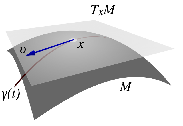
Figure 7: A tangent space \(T_x M\) for manifold \(M\) with tangent vector \({\bf v} \in T_x M\), along a curve travelling through \(x \in M\) (source: Wikipedia).

I should note that Figure 7 is a bit misleading because the tangent space/vector doesn't necessarily look literally like a plane tangent to the manifold. It can however look like this when it is embedded in a higher dimension space like it is here for visualization purposes (e.g. 2D manifold as a surface shown in 3D with a plane tangent to the surface representing the "tangent space"). Manifolds don't need to even be embedded in a higher dimensional space (recall that they are defined just as special sets with a mapping to Euclidean space) so we should be careful with some of these visualizations. However, it's always good to have an intuition. Let's try to formalize this idea in two steps: the first step is a bit more intuitive, the second step is a deeper look to allow us to perform more operations.

Tangent Spaces as the Velocity of Curves

Suppose we have our good old smooth manifold \(M\) and a point on that curve \(p \in M\) (we switch to the variable \(p\) for our point instead of \(x\) because we'll use \(x\) for something else). Recall we have a coordinate chart \(\varphi: U \rightarrow \mathbb{R}^n\) where \(U\) is an open subset of \(M\) containing \(p\). So far so good, this is just repeating what we had in Figure 4.

Now let's define a smooth parametric curve \(\gamma: t \rightarrow M\) that maps a parameter \(t \in [a,b]\) to \(M\) that passes through \(p\). Basically, this just defines a curve that runs along our manifold. Now we want to imagine we're walking along this curve in the local coordinates i.e. after applying our chart (this is where Figure 7 might be misleading), this will give us: \(\varphi \circ \gamma: t \rightarrow \mathbb{R}^n\) (from \(t\) to \(M\) to \(\mathbb{R}^n\) in the local coordinates).

Let's label our local coordinates as \({\bf x} = \varphi \circ \gamma(t)\), which is nothing more than a vector valued function of a single parameter which can be interpreted as your "position" vector on the manifold (in local coordinates) as a function of time \(t\). Thus, the velocity is just the instantaneous rate of change of our position vector with respect to time. So at time \(t=t_0\) when we're at the point \(p\), we have:

\begin{equation*} \text{"velocity" at } p = \frac{d \varphi \circ \gamma(t)}{dt}\Big|_{t=t_0} = \Big[\frac{dx^1(t)}{dt}, \ldots, \frac{dx^n(t)}{dt}\Big]\Big|_{t=t_0} \tag{7} \end{equation*}

where \(x^i(t)\) is the \(i^{th}\) component of our curve in local coordinates (not an exponent). In this case the tangent vector \(\bf v\) is nothing more than the "velocity" at \(p\). If we then take every possible velocity at \(p\) (by specifying different parametric curves) then these velocity vectors make a tangent space, denoted by \(T_pM\) (careful, our point on the manifold is now \(p\) and the local coordinate is \(x\)). Now that we have our tangent (vector) space represented in \(\mathbb{R}^n\), we can perform our usual Euclidean vector-space operations.

Basis of the Tangent Space

Tangent vectors as velocities only tell half the story though because we have a tangent vector specified in a local coordinate system but what is its basis? Recall a vector has its coordinates (an ordered list of scalars) that correspond to particular basis vectors. This is important because we want to be able to do analysis on the manifold between points and charts, not just at a single point/chart. So understanding how the tangent spaces relate between different points (and potentially charts) on a manifold is important.

To understand how to construct the tangent space basis, let's first define an arbitrary function \(f: M \rightarrow \mathbb{R}\) and assume we still have our good old smooth parametric curve \(\gamma: t \rightarrow M\). Now we want to look at a new definition of "velocity" relative to this test function: \(\frac{df \circ \gamma(t)}{dt}\Big|_{t=t_0}\) at our point on the manifold \(p\). Basically the rate of change of our function \(f\) as we walk along this curve.

However, we can do a "trick" by introducing a chart (\(\varphi\)) and its inverse (\(\varphi^{-1}\)) into this measure of "velocity":

\begin{align*} \frac{df \circ \gamma(t)}{dt}\Big|_{t=t_0} &= \frac{d(f \circ \varphi^{-1} \circ \varphi \circ \gamma)(t)}{dt}\Big|_{t=t_0} \\ &= \frac{d((f \circ \varphi^{-1}) \circ (\varphi \circ \gamma))(t)}{dt}\Big|_{t=t_0} \\ &= \sum_i \frac{\partial (f \circ \varphi^{-1})(x)}{\partial x_i}\Big|_{x=\varphi \circ \gamma(t_0)} \frac{d(\varphi \circ \gamma)^i(t)}{dt}\Big|_{t=t_0} && \text{chain rule} \\ &= \sum_i \frac{\partial (f \circ \varphi^{-1})(x)}{\partial x_i}\Big|_{x=\varphi(p)} \frac{d(\varphi \circ \gamma)^i(t)}{dt}\Big|_{t=t_0} && \text{since }p = \gamma(t_0) \\ &= \sum_i (\text{basis for component }i)(\text{"velocity" of component i wrt to } \varphi) \\ \tag{8} \end{align*}

Note the introduction of partial derivatives and summations in the third line, which is just an application of the multi-variable calculus chain rule. We can see that by introducing this test function and doing our little trick we get the same velocity as Equation 7 but with its corresponding basis vectors.

Okay the next part is going to be a bit strange but bear with me. We're going to take the basis and re-write it like so:

\begin{align*} \Big(\frac{\partial}{\partial x^i}\Big)_p (f) := \frac{\partial (f \circ \varphi^{-1})(\varphi(p))}{\partial x_i} \\ \tag{9} \end{align*}

which simply defines some new notation for the basis. Importantly the LHS now has no mention of \(\varphi\) anymore, but why? Well there is a convention that \(\varphi\) is implicitly specified by \(x^i\). So if you have some other chart, say, \(\vartheta\), then you label its local coordinates with \(y^i\). But it's important to remember that when we're using this notation, implicitly there is a chart behind it.

Okay, so now that we've cleared up that, there's another thing we need to look at: what is \(f\)? We know it's some test function that we used, but it was arbitrary. And in fact, it's so arbitrary we're going to get rid of it! So we're just going to define the basis in terms of the operator that acts of \(f\) and not the actual resultant vector! So every tangent vector \(v \in T_pM\), we have:

\begin{align*} {\bf v} &= \sum_{i=1}^n v(x^i) \cdot \Big(\frac{\partial}{\partial x^i}\Big)_p \\ &= \sum_{i=1}^n \frac{d(\varphi \circ \gamma)^i(t)}{dt}\Big|_{t=t_0} \cdot \Big(\frac{\partial}{\partial x^i}\Big)_p \\ \tag{10} \end{align*}

It turns out the basis is actually a set of differential operators, not the actual vectors on the test function \(f\), which make up a vector space! Remember, a vector space doesn't need to be our usual Euclidean vectors, they can be anything that satisfy the vector space properties, including differential operators! A bit mind bending if you're not used to these abstract definitions.

Change of Basis for Tangent Vectors

Now that we have a basis for our tangent vectors, we want to understand how to change basis between them. Let's just setup/recap a bit of notation first. Let's define two charts for our \(d\)-dimensional manifold \(M\):

\begin{align*} \varphi(p) = (x^1(p), \ldots, x^d(p)) \\ \vartheta(p) = (y^1(p), \ldots, y^d(p)) \\ \tag{11} \end{align*}

where \(x^i(p)\) and \(y^i(p)\) are coordinate functions to find the specific index of the local coordinates from a point on our manifold \(p \in M\). Assume that \(p\) is in the overlap of the domains in the two charts. Now we want to look at how we can convert from a tangent space in one chart to another.

(We're going to switch to a more convenient partial derivative notation here: \(\partial_x f := \frac{\partial f}{\partial x}\), which is just a bit more concise.)

So starting from our summation in Equation 10 (and using Einstein summation notation, see also previous my post on Tensors) acting on our test function \(f\):

\begin{align*} {\bf v} f &= v(x^i) \cdot \Big(\frac{\partial}{\partial x^i}\Big)_p f \\ &= v(x^i) \cdot \partial_{x^i} (f \circ \varphi^{-1})(\varphi(p)) && \text{by definition} \\ &= v(x^i) \cdot \partial_{x^i} (f \circ \vartheta^{-1} \circ \vartheta \circ \varphi^{-1})(\varphi(p)) && \text{introduce } \vartheta \text{ with identity trick}\\ &= v(x^i) \cdot \partial_{x^i} ((f \circ \vartheta^{-1}) \circ (\vartheta \circ \varphi^{-1}))(\varphi(p)) \\ &= v(x^i) \cdot \partial_{x^i} (\vartheta \circ \varphi^{-1})^j(\varphi(p)) \cdot \partial_{y^j} (f \circ \vartheta^{-1})(\vartheta \circ \varphi^{-1}(\varphi(p))) && \text{chain rule} \\ &= v(x^i) \cdot \partial_{x^i} (\vartheta \circ \varphi^{-1})^j(\varphi(p)) \cdot \partial_{y^j} (f \circ \vartheta^{-1})(\vartheta(p)) && \text{simplifying} \\ &= v(x^i) \cdot \partial_{x^i} (\vartheta \circ \varphi^{-1})^j(\varphi(p)) \cdot \Big(\frac{\partial}{\partial y^j}\Big)_p f && \text{by definition} \\ &= v(x^i) \cdot \frac{\partial y^j}{\partial x^i}\big|_{x=\varphi(p)} \cdot \Big(\frac{\partial}{\partial y^j}\Big)_p f && \text{since }y^j(x) = y^j(\varphi^{-1}(\varphi(x))) \\ &= v(y^j) \cdot \Big(\frac{\partial}{\partial y^j}\Big)_p f \\ \tag{12} \end{align*}

After some wrangling with the notation, we can see the change of basis is basically just an application of the chain rule. If you squint hard enough, you'll see the change of basis matrix is simply the Jacobian \(J\) of \(\vartheta(x) = (y^1(x), \ldots, y^d(x))\) written with respect to the original chart coordinates \(x^i\) (instead of the manifold point \(p\)). In matrix notation, we would get something like:

\begin{align*} {\bf v(y)} = \begin{bmatrix} v(y^1) \\ \ldots \\ v(y^d) \end{bmatrix} = {\bf J_y} {\bf v(x)} = \begin{bmatrix} \frac{\partial y^1}{\partial x^1}\big|_{x=\varphi(p)} & \cdots & \frac{\partial y^1}{\partial x^d}\big|_{x=\varphi(p)} \\ \vdots & \ddots & \vdots \\ \frac{\partial y^d}{\partial x^1}\big|_{x=\varphi(p)} & \cdots & \frac{\partial y^d}{\partial x^d}\big|_{x=\varphi(p)} \end{bmatrix} \begin{bmatrix} v(x^1) \\ \ldots \\ v(x^d) \end{bmatrix}\\ \tag{13} \end{align*}

For those of you who understand tensors (if not read my previous post Tensors, Tensors, Tensors), the tangent vector transforms contravariantly with the change of coordinates (charts), that is, it transforms "against" the transformation of change of coordinates. A "with" change of coordinates transformation would be multiplying by the inverse of the Jacobian, which we'll see below with the metric tensor.

So after all that manipulation, let's take a look at an example on our sphere to make things a bit more concrete.

Example 4: Tangent Vectors on a Sphere

Let us take the unit sphere, and define a curve \(\gamma(t)\) parallel to the equator at a 45 degree angle from the equator. Figure 8 shows a picture where \(\theta=\frac{\pi}{4}\).

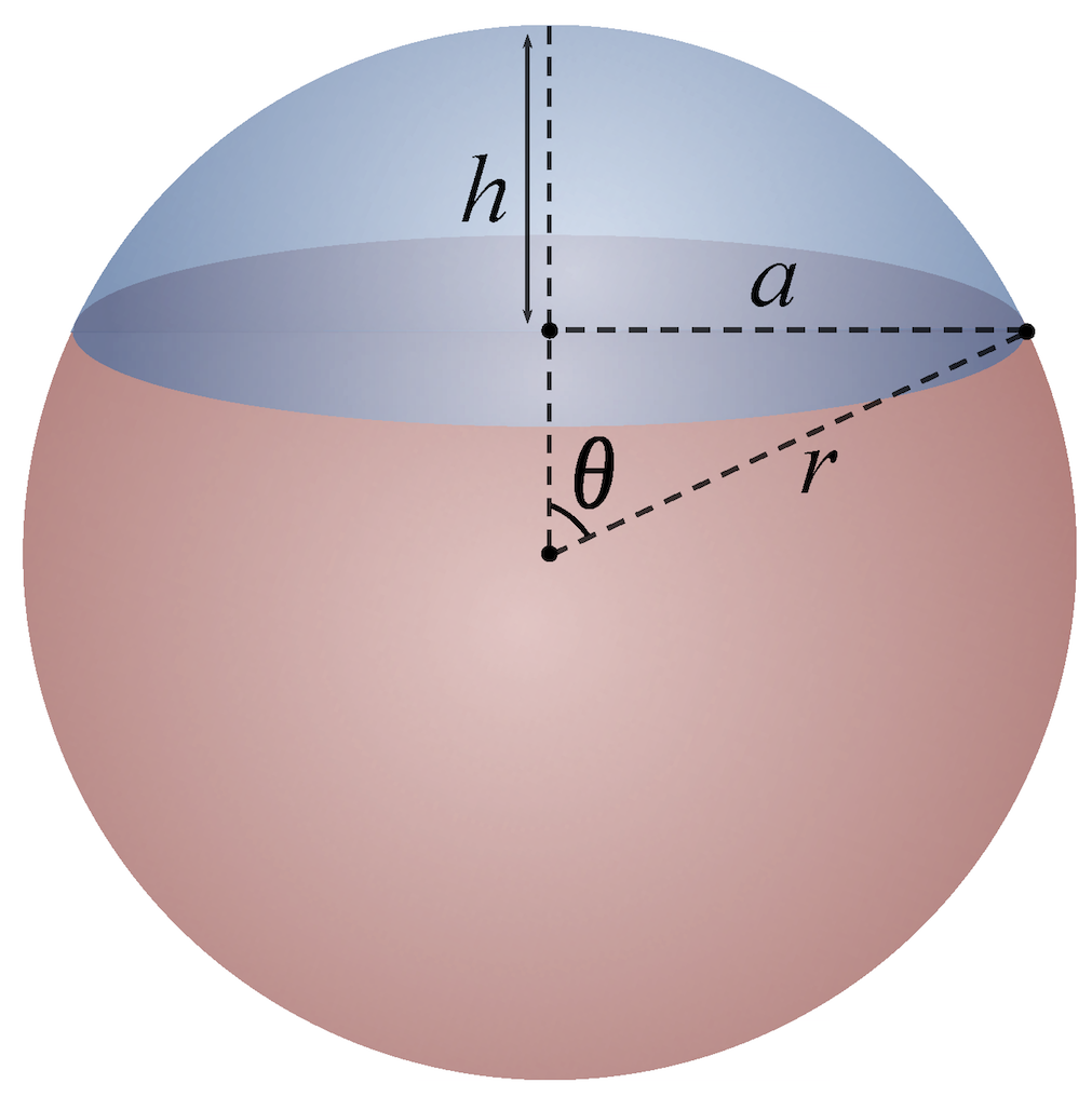
Figure 8: A circle parallel to the equator with angle \(\theta\) (source: Wikipedia).

We can define this parametric curve by:

\begin{equation*} \gamma(t) = (\cos \frac{\pi}{4}\cos\pi t, \cos \frac{\pi}{4}\sin\pi t, \sin \frac{\pi}{4}), \text{ }t \in [-1, 1] \tag{14} \end{equation*}

Notice that the sum of squares of the components of \(\gamma(t)\) equals to \(1\) using the trigonometric identity \(\cos^2 \theta + \sin^2 \theta = 1\). Let's try to find the tangent vector at the point \(p = \gamma(t_0 = 0) = (x, y, z) = (\frac{1}{\sqrt{2}}, 0, \frac{1}{\sqrt{2}})\).

First, following Equation 6, let's write down our chart \(\varphi\) and its inverse (I'm not going to use the superscript notation here for the local coordinates but you should know it's pretty common):

\begin{align*} u_1(x, y, z) &= \frac{x}{1-z} \\ u_2(x, y, z) &= \frac{y}{1-z} \\ x &= \frac{2u_1}{u_1^2 + u_2^2 + 1} \\ y &= \frac{2u_2}{u_1^2 + u_2^2 + 1} \\ z &= \frac{u_1^2 + u_2^2 - 1}{u_1^2 + u_2^2 + 1} \\ \tag{15} \end{align*}

Plugging in our point at \(p=\gamma(t_0=0)\), we get \(\varphi(p) = (u_1, u_2) = (\sqrt{2} + 1, 0)\).

To find the coordinates in our tangent space, we use Equation 7:

\begin{align*} \frac{d \varphi \circ \gamma(t)}{dt}\Big|_{t=t_0} &= \Big[ \frac{d u_1(\cos \frac{\pi}{4}\cos\pi t, \cos \frac{\pi}{4}\sin\pi t, \sin \frac{\pi}{4})}{dt}, \frac{d u_2(\cos \frac{\pi}{4}\cos\pi t, \cos \frac{\pi}{4}\sin\pi t, \sin \frac{\pi}{4})}{dt}, \Big]\Big|_{t=t_0} \\ &= \Big[ \frac{d \big((\sqrt{2} + 1)\cos\pi t\big)}{dt}, \frac{d \big((\sqrt{2} + 1)\sin\pi t\big)}{dt} \Big]\Big|_{t=t_0} \\ &= \Big[ (\sqrt{2}+1)\pi(-\sin\pi t), (\sqrt{2}+1)\pi\cos\pi t \Big]\Big|_{t=t_0} \\ &= (0, (\sqrt{2}+1)\pi) \\ \tag{16} \end{align*}

Combining with our differential operators as our basis, our tangent vector becomes:

\begin{equation*} {\bf T_{\varphi}} = 0 \cdot \big(\frac{\partial}{\partial u_1} \big)_p + (\sqrt{2} + 1)\pi \cdot \big(\frac{\partial}{\partial u_2} \big)_p \tag{17} \end{equation*}

keeping in mind that the basis is actually in terms of the chart \(\varphi\) (implied by the variable \(u_i\)).

Next, let's convert these tangent vectors to our other chart, \(\vartheta\), defined by the south pole (we'll denote the local coordinates with \(w_i\)):

\begin{align*} w_1(x, y, z) &= \frac{x}{1+z} \\ w_2(x, y, z) &= \frac{y}{1+z} \\ x &= \frac{2w_1}{w_1^2 + w_2^2 + 1} \\ y &= \frac{2w_2}{w_1^2 + w_2^2 + 1} \\ z &= \frac{1 - w_1^2 + w_2^2}{w_1^2 + w_2^2 + 1} \\ \tag{18} \end{align*}

Going through the same exercise as above, we can find the tangent vectors with respect to \(\vartheta\) at point \(p\):

\begin{equation*} {\bf T_{\vartheta}} = 0 \cdot \big(\frac{\partial}{\partial w_1} \big)_p + (\sqrt{2} - 1)\pi \cdot \big(\frac{\partial}{\partial w_2} \big)_p \tag{19} \end{equation*}

We should also be able to find \({\bf T_{\vartheta}}\) directly by using Equation 13 and the Jacobian of \(\vartheta\). To do this, we need to find \(w_i\) in terms of \(u_j\):

\begin{align*} w_i(u_1, u_2) &= w_i \circ \varphi^{-1}(u_1, u_2) \\ &= w_i\Big(\frac{2u_1}{u_1^2 + u_2^2 + 1}, \frac{2u_2}{u_1^2 + u_2^2 + 1}, \frac{u_1^2 + u_2^2 - 1}{u_1^2 + u_2^2 + 1} \Big)\\ &= \frac{u_i}{u_1^2 + u_2^2} \tag{20} \end{align*}

Now we should be able to plug the value into Equation 13 to find the same tangent vector by directly converting from our old chart, remembering that \(\varphi(p) = (u_1, u_2) = (\sqrt{2} + 1, 0)\).

\begin{align*} {\bf v(w) } &= {\bf J_u} {\bf v(u)} \\ &= \begin{bmatrix} \frac{\partial w_1}{\partial u_1}\big|_{u=\varphi(p)} & \frac{\partial w_1}{\partial u_2}\big|_{u=\varphi(p)} \\ \frac{\partial w_2}{\partial u_1}\big|_{u=\varphi(p)} & \frac{\partial w_2}{\partial u_2}\big|_{u=\varphi(p)} \end{bmatrix} \begin{bmatrix} 0 \\ (\sqrt{2} + 1)\pi \end{bmatrix}\\ &= \begin{bmatrix} \frac{u_2^2 - u_1^2}{(u_1^2+u_2^2)^2}\big|_{u=\varphi(p)} & -\frac{2u_1u_2}{(u_1^2+u_2^2)^2}\big|_{u=\varphi(p)} \\ -\frac{2u_1u_2}{(u_1^2+u_2^2)^2}\big|_{u=\varphi(p)} & \frac{u_1^2 - u_2^2}{(u_1^2+u_2^2)^2}\big|_{u=\varphi(p)} \end{bmatrix} \begin{bmatrix} 0 \\ (\sqrt{2} + 1)\pi \end{bmatrix}\\ &= \begin{bmatrix} \frac{- (\sqrt{2} + 1)^2}{(\sqrt{2} + 1)^4} & 0 \\ 0 & \frac{(\sqrt{2} + 1)^2}{(\sqrt{2} + 1)^4} \end{bmatrix} \begin{bmatrix} 0 \\ (\sqrt{2} + 1)\pi \end{bmatrix}\\ &= \begin{bmatrix} 0 \\ (\sqrt{2} - 1)\pi \end{bmatrix}\\ \tag{21} \end{align*}

which lines up exactly with our coordinates from Equation 19 above.

Riemannian Manifolds

Even though we now know how to find tangent vectors at each point on a smooth manifold, we still can't do anything interesting yet! To do that we'll have to introduce another special tensor called -- you guess it -- the metric tensor! In particular, the Riemannian metric (tensor) 1 is a family of inner products:

\begin{equation*} g_p: T_pM \times T_pM \rightarrow \mathbb{R}, p \in M \tag{22} \end{equation*}

such that \(p \rightarrow g_p(X(p), Y(p))\) for any two tangent vectors \(X(p), Y(p)\) is a smooth function of \(p\). Note that this is a family of metric tensors, that is, we have a different tensor for every point on the manifold.

The implications of this is that even though each adjacent tangent space can be different (the manifold curves therefore the tangent space changes), the inner product varies smoothly between adjacent points. A real, smooth manifold with a Riemannian metric (tensor) is called a Riemannian manifold. Intuitively, Riemannian manifolds have all the nice "smoothness" properties we would want and makes our lives a lot easier.

Induced Metric Tensors

A natural way to define the metric tensor is to take our \(n\) dimensional manifold \(M\) embedded in \(n+k\) dimensional Euclidean space, and use the standard Euclidean metric tensor in \(n+k\) space but transformed to a local coordinate system on \(M\). That is, we're going to define our family of Riemannian metric tensors using the metric tensor from the embedded Euclidean space. This guarantees that we'll have this nice smoothness property because we're inducing it from the standard Euclidean metric in the embedded space.

To start, let's figure out how to translate a tangent vector in \(n\) dimensional local coordinates back into our \(n+k\) embedding space. Let's use Einstein notation, \(x\) for our embedded space and \(y\) for the local coordinate system with \(y^i(p)\) maps coordinate \(i\) from the embedded space to the local coordinate system, and \(x^i(\varphi(p))\) the reverse mapping. Starting from Equation 10:

\begin{align*} {\bf v} &= v(y^i) \cdot \Big(\frac{\partial}{\partial y^i}\Big)_p \\ &= v(y^i) \cdot \frac{\partial (□ \circ \varphi^{-1})}{\partial y_i}\Big|_{y=\varphi(p)} \\ &= v(y^i) \cdot \frac{\partial x^j}{\partial y^i}\Big|_{y=\varphi(p)} \frac{\partial □}{\partial x^j}\Big|_{x=p} \\ &= v(y^i) \cdot \frac{\partial x^j}{\partial y^i}\Big|_{y=\varphi(p)} \Big(\frac{\partial}{\partial x^j}\Big)_p \\ &= \frac{d \gamma^j(t)}{dt} \cdot {\bf e^j} \\ \tag{23} \end{align*}

I added the "box" symbol there as a placeholder for our arbitrary function \(f\). So here, we're simply playing around with the chain rule to get the final result. The basis is in our embedded space using a similar notation to our local coordinate tangent basis. In fact, we could derive the Equation 23 in the same way as Equation 8 using the "velocity" idea.

Whether in our local tangent space or in the embedded space, they're the same vector (i.e. a tensor). So we could go directly to the velocity \(\frac{d \gamma(t)}{dt}\) instead of doing this back and forth. Additionally, \(\Big(\frac{\partial}{\partial x^j}\Big)_p\) is one-to-one with \(\mathbb{R}^{n+k}\) of our embedded space, so we can also write it in terms of our standard Euclidean basis vectors \({\bf e}^j\) just as well.

Now that we know how to convert between the tangent spaces, we can calculate what our Euclidean metric tensor (i.e. the identity matrix) would be in the local tangent space at point \(p\). Suppose \({\bf v_M}, {\bf w_M}\) are tangent vectors represented in our embedded Euclidean space and \({\bf v_U}, {\bf w_U}\) are the same vectors represented in our local coordinate system:

\begin{align*} g_M({\bf v_M},{\bf w_M}) &= {\bf v_M} \cdot {\bf w_M} && \text{Euclidean inner product}\\ &= \begin{bmatrix} \sum_{i=1}^d v(y^i) \cdot \frac{\partial x^1}{\partial y^i}\Big|_{y=\varphi(p)} & \ldots & \sum_{i=1}^d v(y^i) \cdot \frac{\partial x^n}{\partial y^i}\Big|_{y=\varphi(p)} \end{bmatrix} \begin{bmatrix} \sum_{i=1}^d w(y^i) \cdot \frac{\partial x^1}{\partial y^i}\Big|_{y=\varphi(p)} \\ \ldots \\ \sum_{i=1}^d w(y^i) \cdot \frac{\partial x^n}{\partial y^i}\Big|_{y=\varphi(p)} \end{bmatrix} && \text{Subbing in Equation 23} \\ &= \begin{bmatrix} v(y^1) & \ldots & v(y^d) \end{bmatrix} \begin{bmatrix} \frac{\partial x^1}{\partial y^1}\Big|_{y=\varphi(p)} & \ldots & \frac{\partial x^n}{\partial y^1}\Big|_{y=\varphi(p)} \\ \cdots & \ddots & \cdots \\ \frac{\partial x^1}{\partial y^d}\Big|_{y=\varphi(p)} & \ldots & \frac{\partial x^n}{\partial y^d}\Big|_{y=\varphi(p)} \\ \end{bmatrix} \begin{bmatrix} \frac{\partial x^1}{\partial y^1}\Big|_{y=\varphi(p)} & \ldots & \frac{\partial x^1}{\partial y^d}\Big|_{y=\varphi(p)} \\ \cdots & \ddots & \cdots \\ \frac{\partial x^n}{\partial y^1}\Big|_{y=\varphi(p)} & \ldots & \frac{\partial x^n}{\partial y^d}\Big|_{y=\varphi(p)} \\ \end{bmatrix} \begin{bmatrix} w(y^1) \\ \ldots \\ w(y^d) \end{bmatrix} \\ \tag{24} &= {\bf v_U}^T{\bf J_{x}}^T{\bf J_{x}}{\bf w_U} \\ &= g({\bf v_U}, {\bf w_U}) \\ g_U = {\bf J_{x}}^T{\bf J_{x}} \end{align*}

So we can see that the induced inner product is nothing more than the matrix product of the Jacobian with itself of the mapping from the local coordinate system to the embedded space. Notice that this multiplication by this Jacobian is actually a "with" basis transformation, thus matching the fact that the metric tensor is a (0, 2) covariant tensor. This transformation is opposite of the one we did for tangent vectors in Equation 13, which we can see via the inverse function theorem: \({\bf J_x \circ \varphi} = {\bf (J_y)^{-1}}\).

Now with the metric tensor, you can compute all kinds of good stuff like the length or angle or area. I won't go into all the details of how that works because this post is getting super long. It's very similar to the examples above as long as you can keep track of which coordinate system you are working in.

Conclusion

Whew! This post was a lot longer than I expected. In fact, for some reason I thought I could write a single post on tensors and manifolds, how naive! And the funny part is that I've barely scratched the surface of both topics. This seems to be a common theme on technical topics: you only really see the tip of the iceberg but underneath there is a huge mass of (interesting) details. Differential geometry itself is a much bigger topic than what I presented here and its premier application in special and general relativity. If you search online you'll see that there are some great resources (many of which I used in this post).

In the next post, I'll start getting back to more ML related stuff though. These last two mathematics heavy posts were just a detour for me to pick up a greater understanding of some of the math behind a lot of ML. See you next time!