Hyperbolic Geometry and Poincaré Embeddings

Brian Keng

2018-06-17 08:20

This post is finally going to get back to some ML related topics. In fact, the original reason I took that whole math-y detour in the previous posts was to more deeply understand this topic. It turns out trying to under tensor calculus and differential geometry (even to a basic level) takes a while! Who knew? In any case, we're getting back to our regularly scheduled program.

In this post, I'm going to explain one of the applications of an abstract area of mathematics called hyperbolic geometry. The reason why this area is of interest is because there has been a surge of research showing its application in various fields, chief among them is a paper by Facebook researchers [1] in which they discuss how to utilize a model of hyperbolic geometry to represent hierarchical relationships. I'll cover some of the math weighting more towards intuition, show some of their results, and also show some sample code from Gensim. Don't worry, this time I'll try much harder not going to go down the rabbit hole of trying to explain all the math (no promises though).

(Note: If you're unfamiliar with tensors or manifolds, I suggest getting a quick overview with my previous two posts: Tensors, Tensors, Tensors and Manifolds: A Gentle Introduction)

Curvature

To begin this discussion, we have to first understand something about curvature. There are many different kinds of curvature, and they can be with respect to either curves or surfaces (hypersurfaces) with the latter having many different variants. The basic idea behind all these different definitions is that curvature is some measure by which a geometric object deviates from a flat plane, or in the case of a curve, deviates from a straight line.

As a side note, there can be extrinsic curvature which is defined for objects embedded in another higher dimensional space (usually Euclidean). This means its curvature depends on something (the embedding) besides itself. Alternatively, there is a concept of intrinsic curvature, which is defined in terms of deviation of the surface (or manifold) from flat space. This doesn't depend on any particular embedding but is an "intrinsic" property of the surface (or manifold). We won't go into all the details but the kinds of curvature we'll be talking about will be intrinsic.

Gaussian Curvature

To begin, let's start with Gaussian curvature, which is a measure of curvature for surfaces (2D manifolds). Let's take a look at Figure 1 which shows the three different types of Gaussian curvature.

Figure 1: Examples of the three different types of Gaussian curvature (source: Science4All).

This gives us a good intuition about what it means to have curvature. Starting with the centre diagram (zero curvature), we see that a cylindrical surface has flat or zero curvature in one dimension (blue) and curved around the other dimension (green), resulting in zero curvature. Moving to the right, the sphere on has curvature along its to axis in the same direction, resulting in a positive curvature. And to the left, we see the saddle sheet has curvature along its axis in different directions, resulting in negative curvature. In fact, the Gaussian curvature is the product of its two principal curvatures, which we won't get into detail here but corresponds to our intuition of how a surface curves along its two main axes.

Curvature isn't a uniform property of a surface, it's actually defined point-wise. Figure 2 shows a torus that has all three different types of Gaussian curvature. We won't go deeply into the definition of Gaussian curvature because it's a pain but I think this should probably give some decent intuition on it.

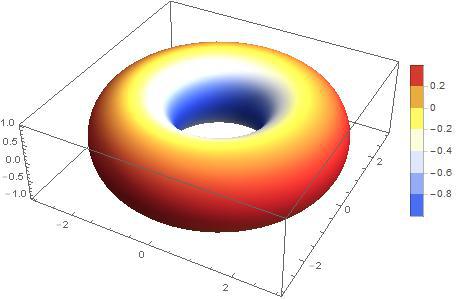
Figure 2: A torus' surface has all three types of curvature. The outside has positive curvature (red); the inside has negative curvature (blue); and a ring on the top and bottom of the torus have zero curvature (yellow-orange) (source: Stackexchange).

Gaussian curvature gives us great intuition on 2D surfaces but what about higher dimensions? The concept of "axes" gets a bit more muddy, so we need an alternate way to define things. One way is to look at the "deviation" of certain geometric objects on the surface (or hypersurface) such as a triangle. Figure 3 shows how a triangle behaves differently on differently curved surfaces.

Figure 3: Deviation of a triangle under the three different types of Gaussian Curvature (source: Science4All).

We can see that in our flat geometry (centre), a triangle's angles add up to exactly \(180^{\circ}\); on positive curvature surfaces (right), it adds up to more than \(180^{\circ}\); on negative curvature surfaces (left), it adds up to less than \(180^{\circ}\). Measuring how an object's properties differs from flat space is (one way) how we're going to generalize curvature to higher dimensions in the next subsection.

Parallel Transport, Riemannian Curvature Tensor and Sectional Curvature

The first idea we need is the concept of parallel transport. The main idea is that we can move tangent vectors along the surface of smooth manifolds to see if our surface is curved.

To illustrate, imagine yourself in a tennis court. First stand in one corner of the tennis court perpendicularly facing the net with your racket parallel to the ground pointing forward (the racket represents the tangent vector). While keeping your racket facing the same direction at all times, walk around the outside tennis court. When you get back to your starting position, the racket is in the same direction (still facing towards the net). This is an example of a flat (or zero curvature) manifold because the vector has not deviated from its original position after "transporting" around this loop.

Now consider another example shown in Figure 4.

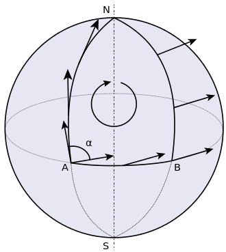
Figure 4: Transporting a tangent vector along the surface of a curved manifold. Notice how the direction of the vector changes when travelling from A to N to B back to A (source: Wikipedia).

From Figure 4, imagine now that we're on the surface of the earth at point A with our racket still parallel to the ground, facing north (i.e. our tangent vector). We walk straight all the way up to the north pole at N, then without changing the direction of our racket, we move towards point B from the north pole. Again, without changing our racket direction, we walk back to point A. This time though, our racket is pointing in a different direction?! This is an example of a curved surface because when we parallel transported the vector, it changed directions.

We can measure this deviation of parallel transport using the Riemannian Curvature Tensor. Starting from a point and moving a vector around a loop, this tensor directly measures the failure of the vector to point in the initial direction. For each point on a smooth manifold, it provides a (1, 3)-tensor, which can be represented as a 4-axis multi-dimensional array. Another way to look at it is that for any two vectors defining a tangent space, it returns a linear transformation that describes how the parallel transport deviates a vector in the tangent space. Note: Since we have a different tensor for each point, the curvature is a local phenomenon.

The math for curvature is quite involved because we're not in flat space anymore. This means we need to setup a lot of additional structures to deal with the fact that we're moving tangent vectors with different tangent spaces. Basically, I'm going to gloss over these details which are beyond the scope of this post (and not to mention my current understanding) :p

Once we have this curvature tensor, we can come up with a measure of curvature called the sectional curvature at a point \(P\) denoted by \(K(u, v)\):

\begin{equation*} K(u, v) = \frac{\langle R(u, v)v, u\rangle }{\langle u, u\rangle \langle v, v\rangle - \langle u, v\rangle ^2} \tag{1} \end{equation*}

where \(u, v\) are linearly independent vectors in the tangent space of point \(P\), \(R\) is the Riemannian Curvature Tensor, and the angle brackets are the inner product.

Manifolds with Constant Sectional Curvature

Riemannian manifolds with constant curvature at every point are special cases of curved surfaces. They come in three forms, which implicitly define three geometries:

Constant Positive Curvature: Elliptic geometry
Constant Zero Curvature: Euclidean geometry
Constant Negative Curvature: Hyperbolic geometry

The first two we are more familiar with: The standard model for Euclidean geometry is just any Euclidean space. The standard model for elliptic geometry is simply just a sphere (or hypersphere). The model for hyperbolic geometry is a bit more complicated and we'll spend some more time with it in the next section.

Euclidean and Non-Euclidean Geometries

We saw above about how constant sectional curvature can be used to induce different types of geometries. But what does this mean? Let's dig in a bit.

If we go way back to Euclid in his seminal work Elements, he gives five postulates (or axioms):

A straight line segment can be drawn joining any two points.
Any straight line segment can be extended indefinitely in a straight line.
Given any straight line segment, a circle can be drawn having the segment as radius and one endpoint as center.
All right angles are congruent.
If two lines are drawn which intersect a third in such a way that the sum of the inner angles on one side is less than two right angles, then the two lines inevitably must intersect each other on that side if extended far enough. (aka the parallel postulate shown in Figure 5)

Figure 5: Euclid's Parallel Postulate: If two lines are placed over a third such that the sum of angles (\(\alpha+\beta\)) are less than two right angles, then they must intersect at some point (source: Wikipedia).

These postulates define Euclidean geometry which is a axiomatic system. An axiomatic system is one in which every theorem can be logically derived from it. This is all jargon relating to logic. So the standard geometry we learn in grade school with lines, circles, angles, etc. is Euclidean geometry.

However, this is not exactly the same thing as the analytical geometry we study when we first learn about the Euclidean plane (i.e. \(\mathbb{R}^2\)). The Euclidean plane (and by extension Euclidean space) is a model of Euclidean geometry:

A model for an axiomatic system is a well-defined set, which assigns meaning for the undefined terms presented in the system, in a manner that is correct with the relations defined in the system.

For example, Euclidean geometry defines a point but there is no concrete meaning to it. In the Euclidean plane, we could define a point as a pair of real numbers \((x,y)\) with \(x,y \in \mathbb{R}\). You could do the same with a line, circle and even an angle (in terms of the metric tensor). Once we concretely define all these abstract things in Euclidean geometry, we have a model of Euclidean geometry. Non-Euclidean geometries can be defined by similar postulates. In particular, by modifying the parallel postulate, we can derive other types of geometries.

Elliptic Geometry

In Elliptic geometry, we change the parallel postulate to:

Two lines perpendicular to a given line must intersect.

where a visualization in shown in Figure 6.

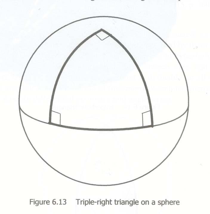
Figure 6: Two lines perpendicular to another line in Elliptic geometry, must intersect at some point (source).

A model of Elliptic geometry is a manifold defined by the surface of a sphere (say with radius=1 and the appropriately induced metric tensor). We can see that the Elliptic postulate holds, and it also yields different theorems than standard Euclidean geometry, such as the sum of angles in a triangle is greater than \(180^{\circ}\).

Hyperbolic Geometry

In Hyperbolic geometry, we change the parallel postulate to:

For any given line R and point P not on R, in the plane containing both line R and point P there are at least two distinct lines through P that do not intersect R.

where a visualization in shown in Figure 7.

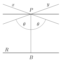
Figure 7: Lines \(x\) and \(y\) intersecting at \(P\) never pass through line \(R\), although it is possible that they can asymptotically approach it (source).

This figure is not a great visualization because, as we'll mention below, you can't really intuitively represent 2D hyperbolic geometry in 2D or 3D Euclidean space. This makes it hard to visualize, and results in a more complex model than the other two geometries. Further down, we'll describe a couple of models of hyperbolic geometry because there is no one "standard" model as we'll see below.

Hyperbolic Space

Hyperbolic space is a type of manifold with constant negative (sectional) curvature. Formally:

Hyperbolic n-space (usually denoted \(\bf H^n\)), is a maximally symmetric, simply connected, n-dimensional Riemannian manifold with constant negative sectional curvature.

Hyperbolic space analogous to the n-dimensional sphere (which has constant positive curvature). This is a very hard thing to visualize though because we're used to only imagining objects in Euclidean space -- not curved space. One way to think about it is that when embedded into Euclidean space, every point is a saddle point... still kind of hard to imagine though. The real tough part is that even for the 2D hyperbolic plane, we cannot embed it into 3D Euclidean space (Hilbert's theorem), so something's got to give.

Fortunately, we can embed models of 2D hyperbolic geometry into a pseudo-Euclidean space called Minkowski space. Interestingly, Minkowski space and curved space in general has applications in special relativity and general relativity, respectively. Let's see how this works.

Minkowski Space

Before we get to the model of hyperbolic geometry, we have to set a few things up. The first thing is what's called a (generalized) Minkowski space (a type of pseudo-Riemannian manifold):

For \(n \geq 2\), a \(n\)-dimensional Minkowski space is a real vector space of real dimension \(n\) which there is a constant Minkowski metric of signature (n-1, 1) or (1, n-1).

Even though it's defined as a vector space, we can regard it as basically having \(n\) real dimensions (just like \(\mathbb{R}^n\)) but with a special type of metric tensor (generalization of dot product): the Minkowski metric. This is where it gets a bit "mind-bending".

The Minkowski metric is not too different from the standard Euclidean metric tensor. For two vectors \({\bf u}=(u_1, \ldots, u_n)\) and \({\bf v} = (v, \ldots, v_n)\), we have:

\begin{align*} g_E({\bf u, v}) &= u_1 v_1 + u_2 v_2 + \ldots + u_n v_n && \text{Euclidean Metric} \\ g_M({\bf u, v}) &= \pm [u_1 v_1 - u_2 v_2 - \ldots - u_n v_n] && \text{Minkowski Metric} \\ \tag{2} \end{align*}

Notice that dimension 1 is treated differently 1 (alternatively dimension 2 to n are different). In special relativity, dimension 1 is considered the "time"-like dimension while the others are "space"-like dimensions. But I don't think this helps with the intuition all that much. For now, we just need to know that one of the dimensions is treated differently, while the others are very similar to our regular Euclidean space.

Hyperboloid

The next thing we need to set up is the hyperboloid. A hyperboloid is a generalization of a hyperbola in two dimensions. If you take a hyperbola and spin it around its principal axes (or add certain types of affine transformations), you get a hyperboloid. There are a few types of hyperboloids but we'll only be talking about the two sheet variant. Figure 8 shows an example of a two sheet hyperboloid.

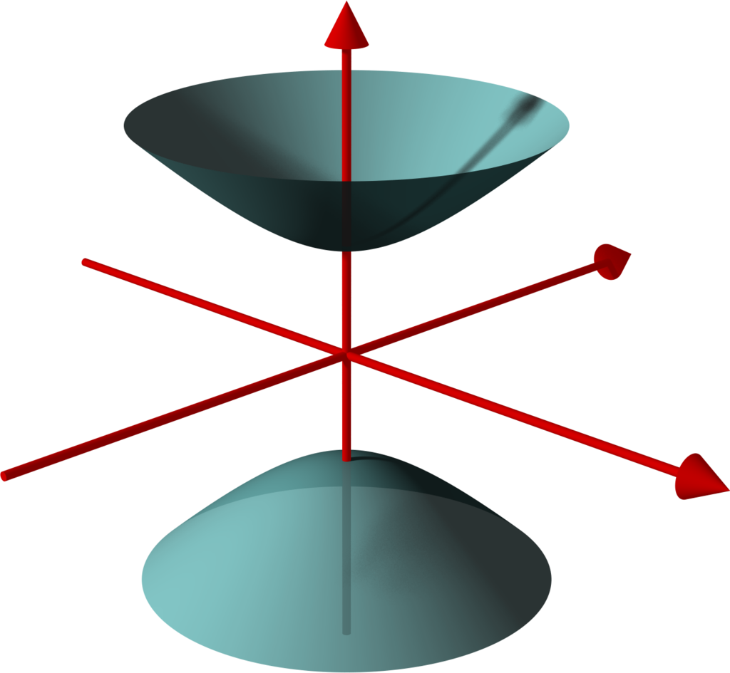
Figure 8: Example of two sheet hyperboloid (source: Wikipedia).

The two sheet hyperboloid (in three dimensions) has the following equation:

\begin{equation*} \frac{x^2}{a^2} + \frac{y^2}{b^2} - \frac{z^2}{c^2} = -1 \tag{3} \end{equation*}

where \(z > 0\) define what is called the "forward sheet". You can see how this can easily extend to multiple dimensions: you just add more positive quadratic terms in front, with your "special" negative dimension (in this case \(z\)) in the back.

A common parametric representation with parameter \(t\) of the two sheet hyperboloid is:

\begin{align*} x &= a\sinh t \cos\theta \\ y &= b\sinh t \sin\theta \\ z &= \pm c\cosh t \\ \tag{4} \end{align*}

Notice that we're using the hyperbolic functions here, which are very much related to hyperbolas (as expected). Also notice that we use \(\cos\theta\) and \(\sin\theta\) for \(x\) and \(y\), which reminds us of the parameterization of a circle. Indeed, x and y are the "normal" Euclidean dimensions and, for a given constant \(z\), they define a circle.

The Hyperboloid Model of Hyperbolic Geometry

Finally we get to our first model of hyperbolic geometry! Having introduced the above two concepts, our first model known as the hyperboloid model (aka Minkowski model or Lorentz model) is a model of n-dimensional hyperbolic geometry in which points are represented on the forward sheet of a two-sheeted hyperboloid of (n+1)-dimensional Minkowski space. The points on this sheet (in 3D Minkowski space) are defined by:

\begin{equation*} x^2 + y^2 - z^2 = -1 \tag{5} \end{equation*}

where \(z>0\). Simple right? Well in case it's not, let's try to add some intuition.

So we know 2D Elliptic geometry (constant positive curvature) can be mapped to a sphere in 3D Euclidean space. So we can re-create any of our usual geometric concepts and have them map to the sphere, for example, points, lines, angles, circles etc. In a similar way for hyperbolic geometry, we can have the same concepts (e.g. points, lines, angles, circles) but mapped to the surface of the forward sheet of the hyperboloid. The big difference is that now we're in Minkowski space which makes your intuition about what should happen a bit screwy.

For example, how does a straight line get defined? On a sphere there are many paths you could take from point A to B, but the shortest path "line" between two points is called a geodesic: the path you take between two points when slicing through the center of the sphere (i.e. a great circle). A geodesic is the generalization of a straight line to curved space, defined to be a curve where you can parallel transport a tangent vector without deformation.

In our hyperboloid model, the geodesic (or our hyperbolic line) is defined to be the curve created by intersecting the plane defined by two points (that define the line) and the origin (i.e. coordinate \((0, 0, 0)\)) with the hyperboloid. So you end up having to go "down" first then back up to reach a point, never just directly towards it using the shortest path on the surface in Euclidean space (which would be around the circumference). Figure 9 shows a visualization of this curve as the brownish line (ignore the bottom circle for now, we'll come back to this later).

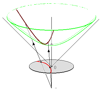
Figure 9: Hyperboloid Stereoscopic Projection (source: Wikipedia).

Once we have the concept of a line segment, we can define the distance between two points. This can be calculated using the arc length of the tangent vectors with the Minkowski metric. This is analogous to how we can compute the length of a curve in Euclidean space, basically walking along it and adding up the infinitesimal distances, except now we'll be using the Minkowski metric from Equation 2. It turns out that this simplifies to a closed form for the hyperbolic distance between two points \(\bf u\) and \(\bf v\):

\begin{equation*} d({\bf u, v}) = arcosh(g_M({\bf u, v})) \tag{6} \end{equation*}

where we're using the inverse (or arc) hyperbolic cosine function and the Minkowski metric defined above.

Example: Calculating the Arc Length of a Geodesic In Hyperbolic Space

To illustrate a few of the above ideas and to gain some intuition, let's calculate the arc length of two points on the hyperbolic plane embedded in 3D Minkowski space. First, let's define a curve from A to B parameterized by \(t=[t_a, t_b]\). We'll pick a simple curve that lies on the plane \(y=0\) (i.e. setting \(\theta=0\) in Equation 4):

\begin{align*} x &= \sinh t \\ y &= 0 \\ z &= \cosh t \\ \tag{7} \end{align*}

Computing the arc length on a manifold, we have:

\begin{align*} d(A, B) &= \int_{t_a}^{t_b} \sqrt{ g_M\big( (\frac{dx(t)}{dt}, \frac{dy(t)}{dt}, \frac{dz(t)}{dt}), (\frac{dx(t)}{dt}, \frac{dy(t)}{dt}, \frac{dz(t)}{dt}) \big)} dt \\ &= \int_{t_a}^{t_b} \sqrt{ \big(\frac{dz(t)}{dt}\big)^2 - \big(\frac{dx(t)}{dt}\big)^2 - \big(\frac{dy(t)}{dt}\big)^2 } dt \\ &= \int_{t_a}^{t_b} \sqrt{ \big(\frac{d \cosh t}{dt}\big)^2 - \big(\frac{d \sinh t}{dt}\big)^2 } dt \\ &= \int_{t_a}^{t_b} \sqrt{ \sinh^2 t -\cosh^2 t } dt \\ &= \int_{t_a}^{t_b} \sqrt{ 1 } dt \\ &= t_b - t_a \\ \tag{8} \end{align*}

This should match up to Equation 6. Let's see what happens:

\begin{align*} d(A, B) &= arcosh\Big(g_M\big( (\sinh t_a, 0, \cosh t_a), (\sinh t_b, 0, \cosh t_b), \big) \Big) \\ &= arcosh(\cosh t_a \cosh t_b - \sinh t_a \sinh t_b) \\ &= arcosh(cosh(t_b - t_a)) && \text{hyperbolic identity} \\ &= t_b - t_a \\ \tag{9} \end{align*}

As expected, the Equation 6 properly calculates the arc length with the Minkowski metric in this case.

The hyperboloid model also has the concept of circles. The simplest circle is with center perpendicular at the bottom most point of the hyperboloid, \((0, 0, 1)\). The circles created with this center look like regular circles in Euclidean space where the circle is on a plane parallel to the \(z=0\) plane. The points on this circle are a constant hyperbolic distance away from this bottom point.

However, if we move to points centered at different locations, we get arbitrary "slices" of the hyperboloid as shown in Figure 10 as an ellipse. The non-Euclidean nature of the distance makes it so that the center of this hyperbolic circle is somewhere on the hyperboloid (not a point floating in the middle as you would intuitively expect in Euclidean geometry). This point should be equi-hyperbolic distance from the ellipse created from the "slice".

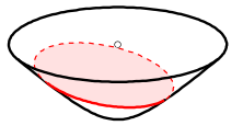
Figure 10: Visualization of a hyperboloid circle as a "slice" of the forward sheet of a hyperboloid (source: Wikipedia).

So that's a quick overview of our first model of hyperbolic geometry. Although "easy" to understand because it's an extension of some concepts we're familiar with, we want to actually just use this as a stepping stone to get to our next model of hyperbolic geometry: the Poincaré ball model.

Poincaré Ball Model

The Poincaré ball model is a model of n-dimensional hyperbolic geometry in which all points are embedded in an n-dimensional sphere (or in a circle in the 2D case which is called the Poincaré disk model). This is being presented second because it is much less intuitive but can be derived directly from the hyperboloid model.

Can a circle fit an entire geometry?

You might be wondering how we can "fit" an entire geometry in a circle. We know flat 2D geometry fits in the Euclidean plane, 2D elliptic geometry (constant positive curvature) fits on the surface of a sphere, and now we're saying 2D hyperbolic geometry fits inside a circle? The biggest thing to realize is, first, there are an infinite number of points within the circle -- infinities are hard to reason about. Second, we need to throw away our Euclidean sensibilities and intuition. For example, we'll see below that the "distance" between points grows exponentially as we move towards the outside of the Poincaré disk. We need to use a combination of the math and throwing away our old intuition in order to understand these non-flat models of geometry.

The Poincaré model can be derived using a stereoscopic projection of the hyperboloid model onto the unit circle of the \(z=0\) plane. We'll stick with the 2D case but the same ideas can be extended into higher dimensions. Figure 11 shows a visualization.

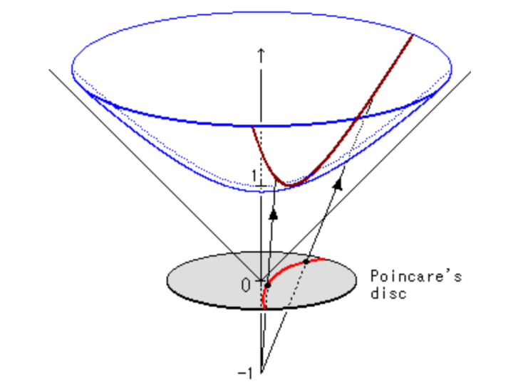
Figure 11: Stereoscopic projection to derive the Poincaré Disk Model (source: inspirehep.net).

The basic idea of this stereoscopic projection (in 3D but this idea generalizes) is:

Start with a point \(P\) on the hyperboloid we wish to map.
Extend \(P\) out to a focal point \(N=(0, 0, -1)\) to form a line.
Project that line onto the \(z=0\) plane to find our point \(Q\) in the Poincaré model.

If you do the algebra, you'll find the following equations for point \(P=(x_1, \ldots, x_n, z)\) on the hyperboloid and \(Q=(y_1, \ldots, y_n)\) in the unit circle of the \(z=0\) plane:

\begin{align*} y_i &= \frac{x_i}{z + 1} \\ (z, x_i) &= \frac{(1 + \sum y_i^2, 2y_i)}{1 - \sum y_i^2} \\ \tag{10} \end{align*}

As with our other hyperbolic model, we can represent common geometric concepts by points on the unit circle. Starting with a line, if we project the geodesic line from the hyperboloid to the unit circle, we get an arcs along the unit circle as shown in Figure 12.

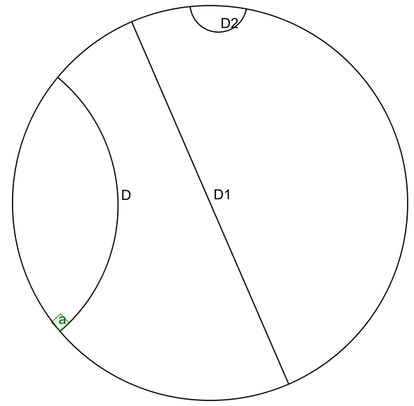
Figure 12: Examples of Poincaré lines as arcs on the unit circle with each one approaching the circumference at a 90 degree angle. (source: Wikipedia)

A few notable points:

The arcs never reach the circumference of the circle. This is analogous to the geodesic on the hyperboloid extending out the infinity, that is, as the arc approaches the circumference it's approaching the "infinity" of the plane.
This means distances at the edge of the circle grow exponentially as you move toward the edge of the circle (compared to their Euclidean distances).
Each arc approaches the circumference at a 90 degree angle, this just works out as a result of the math of the hyperboloid and the projection. The straight line in this case is a point that passes through the "bottom" of the hyperboloid \((0, 0, 1)\).
In this case, we can see 3 lines that are parallel and actually diverge from each other (also known as "ultra parallel"). This is a consequence of changing Euclid's fifth postulate regarding parallel lines (see the box above). A more clear example is Figure 13. Here we see that we can have an infinite number of lines (black) intersecting at a single point and still be parallel to another line (blue).

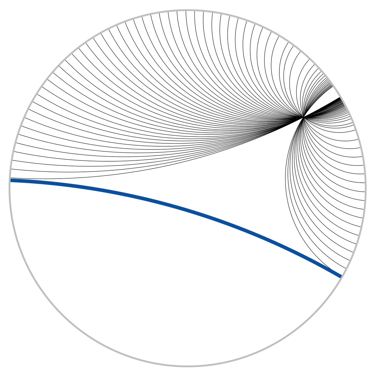
Figure 13: Hyperbolic parallel lines that do not intersect on the Poincaré disk. (source: Wikipedia)

The distance the two points can be computed in the same way as the hyperboloid, namely, taking the integral over the arc of line element (defined by the associated metric tensor). If we remember our differential geometry, we can actually derive the Poincaré disk metric tensor from the hyperboloid model using our transformations from Equation 10. I'll show a partial derivation here (you can work out all the algebra as an exercise :p). Starting with the line element calling our hyperboloid variables \(x_1,x_2,z\) and our Poincaré disk variables \(y_1, y_2\):

\begin{align*} ds^2 &= \begin{bmatrix} dx_1 & dx_2 & dz \end{bmatrix} \begin{bmatrix} 1 & 0 & 0 \\ 0 & 1 & 0 \\ 0 & 0 & -1 \\ \end{bmatrix} \begin{bmatrix} dx_1 \\ dx_2 \\ dz \end{bmatrix} && \text{Minkowski metric} \\ &= \begin{bmatrix} dy_1 & dy_2 \end{bmatrix} \begin{bmatrix} \frac{\partial x_1}{\partial y_1} & \frac{\partial x_2}{\partial y_1} & \frac{\partial z}{\partial y_1} \\ \frac{\partial x_1}{\partial y_2} & \frac{\partial x_2}{\partial y_2} & \frac{\partial z}{\partial y_2} \end{bmatrix} \begin{bmatrix} 1 & 0 & 0 \\ 0 & 1 & 0 \\ 0 & 0 & -1 \\ \end{bmatrix} \begin{bmatrix} \frac{\partial x_1}{\partial y_1} & \frac{\partial x_1}{\partial y_2} \\ \frac{\partial x_2}{\partial y_1} & \frac{\partial x_2}{\partial y_2} \\ \frac{\partial z}{\partial y_1} & \frac{\partial z}{\partial y_2} \end{bmatrix} \begin{bmatrix} dy_1 \\ dy_2 \end{bmatrix} && \text{total differential}\\ &= \ldots && \text{sub in Equation 10} \\ &= \begin{bmatrix} dy_1 & dy_2 \end{bmatrix} \begin{bmatrix} \frac{4}{(1 - y_1^2 - y_2^2)^2} & 0 \\ 0 & \frac{4}{(1 - y_1^2 - y_2^2)^2} \end{bmatrix} \begin{bmatrix} dy_1 \\ dy_2 \end{bmatrix} \\ &= \frac{4 \lVert{\bf dy}\rVert^2}{(1-\lVert{\bf y}\rVert^2)^2} \\ \tag{11} \end{align*}

If you go through the exercise of finding the arc-length using this metric, we'll find the distance between two points \(u,v\) on the Poincaré ball is given by:

\begin{align*} d(u,v) = arcosh\big(1 + 2\frac{\lVert u-v \rVert^2}{(1-\lVert u\rVert^2)(1-\lVert v\rVert^2)}\big) \\ \tag{12} \end{align*}

where the double bars represent the Euclidean distance. Equation 12 is a bit more complicated than on the hyperboloid but nothing that's not easily computable using standard functions.

A hyperbolic circle defined as a set of points at a constant radius from a center point, is in general any Euclidean circle completely contained within the unit circle. However, the unintuitive part is that the center point is not in general the normal Euclidean center, but rather something asymmetrical. The only time it is the actual Euclidean center is if it's at point (0,0).

Poincaré Visualization

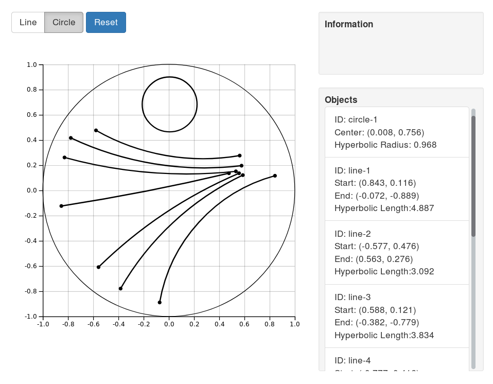
Here's an interactive visualization I made with D3.js, Numeric.js and Bootstrap. You can play around drawing hyperbolic lines and circles. The interesting things to play around with are:

How the same length Euclidean distance maps to different distances on the Poincaré disk.
How a line segment is actually part of a larger circle intersecting the Poincaré disk.
How the Euclidean center of a circle can be very different than its hyperbolic center.

Figure 14: Screenshot of My Poincaré Disk Visualization.

The implementation is all there in the attached JavaScript files. It's pretty much a hack that I put together. JavaScript can be pretty frustrating because of all the little interaction details you have to get right! It's no wonder why I'm not a frontend guy.

The more interesting part (to me) was getting the math right for generating the hyperbolic lines and circles. For generating lines, Wikipedia has a nice little algorithm to generate the hyperbolic line. They're mostly just variations on basic line equations for the most part. Although, it did take me a while to get this mostly right because there are a lot of equations and operations to code. Another lesson learned: it's hard to roll your own numeric calculations! (Better to use a library when available.)

For the circle, I just cheated and used Numeric.js to solve for the points that I needed. The algorithm I used was basically find 3 points that were equidistant from the starting point. The current position of the mouse defines one of them (P1). For the next one, I used the line created from P1 to the starting point to find another one on the opposite side (P2) using Numeric.js. The third point, I used the perpendicular line passing through the starting point (P3), again using Numeric.js. Lastly, I used the formula for finding the equation of a circle from three points and was able to draw the circle!

Poincaré Embeddings for Hierarchical Representations

The Limitations of Euclidean Space for Hierarchical Data

The whole reason why we went through that primer on hyperbolic geometry is that we want to embed data in it! Consider some hierarchical data, such as a tree. A tree with branching factor \(b\) has \((b+1)b^{l-1}\) nodes at level \(l\) and \(\frac{(b+1)b^{l}-2}{b-1}\) nodes on levels less than or equal to \(l\). So as we grow the levels of the tree, the number of nodes grows exponentially.

There are really two important pieces of information in a tree. One is the hierarchical nature of the tree: the parent-child relationships. The other is a relative "distance" between the nodes. Children and their parents should be close, but leaf nodes in totally different branches of the tree should be very far apart (probably somehow proportional to the number of links).

Let's imagine putting this into a Euclidean (say 2D) space. First, we would probably put the root at the origin. Then, place the first level equidistant around it. Then place the second level equidistant from all those points. Figure 15 shows these two levels.

Figure 15: An attempt at embedding a tree with branching factor 4 into the Euclidean plane. We are already starting to run out of space!

You can see we're already running out of space. The hierarchical links are sort of represented (distances between child/parent are maintained), but importantly, the distances between siblings is gets smaller. Look at the leaf nodes which are squeezed at the edge because we don't have enough "space". One way around, might be to increase dimensions but then you'd need to increase those with the number of levels you have, which brings a whole host of other problems. Long story short, Euclidean space isn't a good representation for graph-like data.

Embedding Hierarchies in Hyperbolic Space

It shouldn't be a surprise at this point to know that hyperbolic space is a good representation of hierarchical data ([1]). Using the same sort of algorithm as we tried above of placing the root at the center and spacing the children out equidistant recursively does work in hyperbolic space. The reason is that distances grow exponentially as we move toward the edge of the disk, eliminating the "crowding" effect we saw above. Figure 16 shows a visualization for a tree with branching factor two.

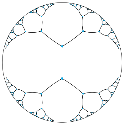
Embedding a hierarchical tree in hyperbolic space

Figure 16: Embedding a hierarchical tree with branching factor two into a 2D hyperbolic plane (Poincaré disk). Distances between all points are actually equal because distances grow exponentially as you move toward the edge of the disk (source: [1]).

Of course, Figure 16 looks crowded at the lower levels just like the previous figure but that's only because hyperbolic space is hard to visualize intuitively. In fact all the points in Figure 16 are equidistant from their parent, and siblings and cousins nodes are much further apart then they appear. So crowding in fact isn't much of an issue (use my visualization above to play around with it). We can also use the exact same idea but instead of the Poincaré disk use the Poincaré ball in \(d\) dimensions.

The problem now becomes, how do I map my nodes in my hierarchical data to the Poincaré ball? As usual, via an optimization. We have to use a variant of our usual stochastic gradient descent called Riemannian Stochastic Gradient Descent (RSGD) because we're optimizing over a manifold, not just simple Euclidean space. I won't go through all the math (partly because I don't quite understand it) but here is the final update equations for the embeddings we want to learn \(\bf \theta\):

\begin{align*} proj({\bf \theta}) &= \begin{cases} \frac{\bf \theta}{\lVert{\bf \theta}\rVert - \epsilon} && \text{if } \lVert {\bf \theta} \rVert \geq 1 \\ {\bf \theta} && \text{otherwise} \end{cases} \\ {\bf \theta_{t+1}} &\leftarrow proj\big({\bf \theta_t} - \eta_t \frac{(1 - \lVert{\bf \theta_t}\rVert^2)^2}{4} \nabla_E\big)\\ \tag{13} \end{align*}

where \(\epsilon\) is a small constant for numerical stability, \(\eta_t\) is the learning rate, and \(\nabla_E\) is our usual (Euclidean) gradient of our loss. The first equation just makes sure we stay within the unit ball. The second equation is our usual parameter SGD updating except with a rescaling of the gradient to account for our hyperbolic distances.

So far we haven't talked about the loss function. That's because in [1], they use a few different ones depending on what they're trying to do. We'll focus on the one used for hierarchical data, which bears a striking resemblance to Word2vec's Skip-Gram loss with negative sampling:

\begin{align*} \mathcal{L}_{\text{paper}}(\Theta) &= \sum_{\substack{(u,v) \in \mathcal{D}}} \log \frac{e^{-d(u,v)}}{\sum_{v'\in \mathcal{N}(u)} e^{-d(u, v')}} \\ \mathcal{L_{\text{impl}}}(\Theta) &= \sum_{\substack{(u,v) \in \mathcal{D}}} \log \frac{e^{-d(u,v)}}{e^{-d(u,v)} + \sum_{v'\in \mathcal{N}(u)} e^{-d(u, v')}} \\ \tag{14} \end{align*}

where \(\mathcal{N}(u)\) is a set of negative samples for \(u\) and \(\mathcal{D}\) is our link dataset. The difference between the two versions (according to [2]) is that the paper gives the former while the actual implementation from [1] gives the latter. Both are very similar, and the testing done in [2] seems to favor the latter.

In either case, from Equation 14, for a given hierarchical link \((u, v)\), we are basically trying to pull them closer (numerator), while pushing a random negative sample of the non-relations apart (denominator). This can be interpreted as a soft ranking loss where \(d(u, v)\) comes before \(d(u, v')\). The negative sampling (just like Word2vec) is really done just for computational feasibility, we could also do it over every non-link if we wanted.

And that's about it! There are actually a few more tricks that [2] uncovered in the original C++ implementation from [1] that practically are important to get a good embedding, I encourage you to check out that blog post, which is very accessible.

Applications and Gensim's Poincaré Implementation

So there are a few tasks that they used to evaluate these hierarchical embeddings in the paper ([1]):

Reconstruction of a hierarchy/graph from the embedding (this is a synthetic test because you use all the data to construct the embedding).
Link prediction with a train/validation/test set.

They show results on three different datasets: transitive closure of WordNet noun hierarchy, social network embeddings, and a lexical entailment dataset. They compare these datasets to standard Euclidean distance and a related "translational" distance using a similar loss function. Here are the reconstruction results from [1] on WordNet:

Figure 17: Experimental results from [1] showing a massive improvement in reconstruction performance.

You can see that the Poincaré embedding shows a massive improvement over the other methods using the average rank and mean average precision. Rank in this context means where did the actual link distance rank relative to all ground truth negative examples. Ideally it should be rank 1. With even as little as 5 dimensions, the Poincaré embeddings massively outperform the two other distance functions with 200 dimension. This really shows the efficiency of the embedding.

What's even nicer about these embedding is that there is a great implementation from Gensim. [2] is a technical post by the authors of Gensim describing how they implemented these embeddings.

The model is trivial to run using Gensim. Here's some sample code from their documentation:

from gensim.models.poincare import PoincareModel
relations = [('kangaroo', 'marsupial'), ('kangaroo', 'mammal'),
             ('gib', 'cat')]
model = PoincareModel(relations, negative=2)
model.train(epochs=50)

I love it when there are nice clean open source implementations available. Coding these up from scratch invariably takes a huge amount of time, especially when you have to reverse engineer an implementation from a paper (at least they had the original authors' C++ implementation though).

Conclusion

Well that's it! Started off with a bunch of math then slowly corrected course back to some ML topics. My next post will definitely be back along the lines of ML, I've had enough of this diversion into the maths. Besides, there are still so many interesting papers and topics for me to look at, it just seems like the backlog keeps growing! Stay tune for some more posts.

(As a side note: It seems my posts keep getting longer and longer. I have got to consciously break them up into smaller pieces, maybe do some "Agile" or "Lean Blogging" on them. Or not. We'll see.)